Why is My Matlab Function Not Providing Critical Points at the Expected Maximum?

In summary: DIn summary, the conversation discusses finding critical points for a function that appears to have a maximum at approximately x=y=5. Through plotting and using code to solve for critical points, it is determined that there are in fact critical points at various coordinates. Using a function called Reduce, more critical points are found and it is concluded that there is a critical point at the red mountain on the graph.
  • #1
FocusedWolf
81
0
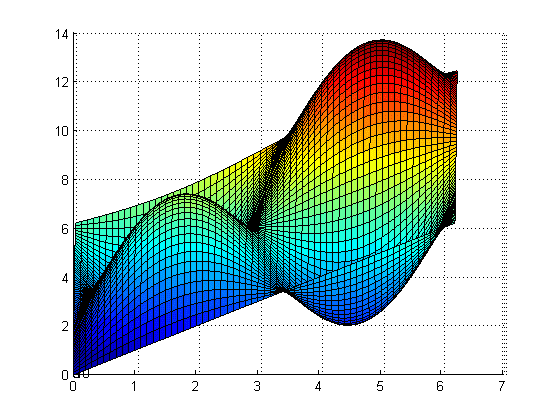
I have a function that is not giving me critical points for where their appears to be a maximum.

from plot their seems to be a cp at approximately x=y=5
plot.png


However, these are the cp's:
cpx =

-0.2618
-1.3090
1.8326
2.8798
-2.8798
-1.8326
1.3090
0.2618cpy =

-0.2618
-1.3090
1.8326
2.8798
0.2618
1.3090
-1.8326
-2.8798

When evaluated on the boundry [0,2pi]x[0,2pi] F(0,0)=0 as a absolute minimum and F(2*pi, 2*pi)=12.5664 as absolute maximum...even though in the graph... 2*pi is lower then the imaginary big red mountain on right...for which their seems to be no cp...

Here's code that generates plot and finds critical points

Code:
%plotting it
[x,y] = meshgrid(0 : .1 : 2*pi)
z = x+y+4.*sin(x).*sin(y)
surf(x,y,z)
%contour(x,y,z,20); axis square; colorbar;

syms x y
f = x+y+4*sin(x)*sin(y)
fx = diff(f,x)
fxx = diff(fx,x)
fy = diff(f,y)
fyy = diff(fy,y)
fxy = diff(fx,y)
d = fxx*fyy-fxy^2

% Solve for all critical points of f using solve
[cpx,cpy] = solve(fx,fy)

% Make critical points decimals
cpx = double(cpx)
cpy = double(cpy)

% Make inline functions for f, fxx, and d
F = inline(vectorize(f),'x','y')
D = inline(vectorize(d),'x','y')
Fxx = inline(vectorize(fxx),'x','y')

% define boundries
%[0 0; 0 2*pi; 2*pi 0; 2*pi 2*pi]
boundx = [0; 0; 2*pi; 2*pi]
boundy = [0; 2*pi; 0; 2*pi]

% Make a table of the cp's, F(at cp's), D(at cp's), and Fxx(at cp's)
T = [cpx cpy F(cpx,cpy) D(cpx,cpy) Fxx(cpx,cpy)]

%Evaluate F at boundries of region [0,2pi]x[0,2pi]
T = [boundx boundy F(boundx,boundy)]

So my question is...is their a cp at that red mountain? or is their no red mountain :P
They say when fx and fy DNE their is also cp...but i don't see that happening since fx and fy are polynomials...
 
Last edited:
Physics news on Phys.org
  • #2
FocusedWolf said:
I have a function that is not giving me critical points for where their appears to be a maximum.

from plot their seems to be a cp at approximately x=y=5
plot.png


However, these are the cp's:
cpx =

-0.2618
-1.3090
1.8326
2.8798
-2.8798
-1.8326
1.3090
0.2618


cpy =

-0.2618
-1.3090
1.8326
2.8798
0.2618
1.3090
-1.8326
-2.8798

When evaluated on the boundry [0,2pi]x[0,2pi] F(0,0)=0 as a absolute minimum and F(2*pi, 2*pi)=12.5664 as absolute maximum...even though in the graph... 2*pi is lower then the imaginary big red mountain on right...for which their seems to be no cp...

Here's code that generates plot and finds critical points

Code:
%plotting it
[x,y] = meshgrid(0 : .1 : 2*pi)
z = x+y+4.*sin(x).*sin(y)
surf(x,y,z)
%contour(x,y,z,20); axis square; colorbar;

syms x y
f = x+y+4*sin(x)*sin(y)
fx = diff(f,x)
fxx = diff(fx,x)
fy = diff(f,y)
fyy = diff(fy,y)
fxy = diff(fx,y)
d = fxx*fyy-fxy^2

% Solve for all critical points of f using solve
[cpx,cpy] = solve(fx,fy)

% Make critical points decimals
cpx = double(cpx)
cpy = double(cpy)

% Make inline functions for f, fxx, and d
F = inline(vectorize(f),'x','y')
D = inline(vectorize(d),'x','y')
Fxx = inline(vectorize(fxx),'x','y')

% define boundries
%[0 0; 0 2*pi; 2*pi 0; 2*pi 2*pi]
boundx = [0; 0; 2*pi; 2*pi]
boundy = [0; 2*pi; 0; 2*pi]

% Make a table of the cp's, F(at cp's), D(at cp's), and Fxx(at cp's)
T = [cpx cpy F(cpx,cpy) D(cpx,cpy) Fxx(cpx,cpy)]

%Evaluate F at boundries of region [0,2pi]x[0,2pi]
T = [boundx boundy F(boundx,boundy)]

So my question is...is their a cp at that red mountain? or is their no red mountain :P
They say when fx and fy DNE their is also cp...but i don't see that happening since fx and fy are polynomials...

Are you solving for fx = fy? Or better yet fx - fy = 0?

I kind of see that in your little problem, but everything after that seems like a blur.

Why don't you just solve the above expression, and check if those critical points are maximums?

I'm not sure if that is exactly what the graph looks like, so I'll assume you did it right. If you did it right, it seems like you do have a maximum. Now the problem is either the program can't solve it or the steps you're following are wrong.
 
  • #3
Yea it looks like it's solving them equal to each other or considering both...same thing. It's how an example i found did it for these sorts of problems.

Mathematica gave same answers for critical points.

Solve[{0.0 == Fx[x, y], 0.0 == Fy[x, y]}, {x, y}]

{{y -> -2.87979, x -> 0.261799}, {
y -> -1.8326, x -> 1.309}, {y -> -1.309, x -> -1.309}, {y -> -0.261799,
x -> -0.261799}, {y -> 0.261799, x -> -2.87979}, {y ->
1.309, x -> -1.8326}, {y -> 1.8326, x -> 1.8326}, {
y -> 2.87979, x -> 2.87979}}
 
  • #4
Hmm i think i got em...was reading some warning messages in mathematica that saying not all solutions may be found cause it was using inverse functions, and to use some function called Reduce...so with a bit of tinkering...

N[Reduce[{0 == Fx[x, y] , 0 == Fy[x, y], 0 ≤ x ≤ 2*\[Pi] , 0 ≤ y ≤ 2*\[Pi]}, {x, y}]]

finds these:

(x == 4.97419 && y == 4.97419) || (x == 6.02139 && y == 6.02139) || (x ==
1.8326 && y == 1.8326) || (
x == 2.87979 && y == 2.87979) || (x == 3.40339 && y == 0.261799) || (x == 4.45059 && y == 1.309) || (x == 0.261799 && y == 3.40339) || (x ==
1.309 && y == 4.45059)

and those look like the cp's i was looking for.
 

What is a Matlab maxima minima problem?

A Matlab maxima minima problem is a type of mathematical optimization problem where the goal is to find the maximum or minimum value of a function within a given set of constraints. This is commonly used in various fields of science, engineering, and economics.

How can I solve a Matlab maxima minima problem?

There are several approaches to solving a Matlab maxima minima problem, including using built-in functions like fminbnd or fmincon, or creating your own custom algorithm using a combination of mathematical techniques such as gradient descent and constrained optimization.

What are the common applications of Matlab maxima minima problems?

Matlab maxima minima problems have a wide range of applications in various fields, such as finding the optimal production schedule in manufacturing, determining the most profitable investment portfolio, and identifying the fastest route for a vehicle to travel.

What is the difference between a local and global maxima or minima?

A local maxima or minima refers to the highest or lowest point in a specific region of a function, while a global maxima or minima is the highest or lowest point in the entire function. In other words, a global maxima or minima is the absolute highest or lowest value, while a local maxima or minima may only be the highest or lowest value within a smaller range of the function.

How can I determine if a solution to a Matlab maxima minima problem is valid?

To determine the validity of a solution, you can use the second derivative test or the first derivative test, depending on the type of problem. These tests can help determine if the solution is a maximum or minimum, or if it is neither and therefore not a valid solution.

Similar threads

  • Calculus and Beyond Homework Help
Replies
2
Views
1K
  • Calculus and Beyond Homework Help
Replies
3
Views
3K
  • Calculus and Beyond Homework Help
Replies
4
Views
1K
Replies
1
Views
832
  • Calculus and Beyond Homework Help
Replies
5
Views
2K
  • Calculus and Beyond Homework Help
Replies
5
Views
6K
  • Calculus and Beyond Homework Help
Replies
3
Views
3K
  • Calculus and Beyond Homework Help
Replies
8
Views
2K
  • Calculus and Beyond Homework Help
Replies
9
Views
2K
  • Calculus and Beyond Homework Help
Replies
3
Views
2K
Back
Top