Solving the heat equation with complicated boundary conditions

In summary, the conversation discusses the difficulty in solving a transient problem with specified heat flux boundary conditions that are dependent on the unknown temperatures at the boundaries. The conversation also mentions different approaches to solving the problem and potential simplifications that can be made. The expert offers to help find a solution through approximations or numerical methods and asks for specific parameters of the problem.
  • #1
womfalcs3
62
5
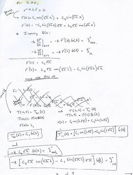
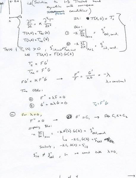
Hi, it is easy solving these PDEs with the idealized homogeneous BCs they throw out in class, but I am having some difficulty solving the transient problem posed in the images below. I have tried working through it, but I don't have confidence in the result. I overlook the solution when the eigenvalues are 0 because that results in the derivative boundary conditions having to equal each other at all times, which is not true for the problem at hand. I also took the cosh and sinh route when the the eigenvalues are negative, but that was giving me similar C1 and C2 formulations as when the eigenvalues are positive. May I please get some direction as to where I'm going wrong? Does the end result make sense? I don't mind not solving for eigenvalues now as the intention is to have a symbolic representation.

Thank you very much.
34qs1gg.jpg


2d8p5jc.jpg


s64wlz.jpg
 
Physics news on Phys.org
  • #2
I'm confused about the boundary conditions. Are you specifying the temperatures at the two boundaries as functions of time, or the heat fluxes at the two boundaries?

Chet
 
  • #3
The actual boundary conditions of interest specify the heat fluxes; however, the heat fluxes are dependent on the temperatures on the boundaries, which are also unknown.

I just also include T(0,t) and T(L,t) being non-zero and positive. Is it wrong of me to impose those Dirichlet conditions in the solution process?

Thanks.


EDIT: I have tried to resolve it using only the derivative conditions: What irks me is that G(t) disappears, which means the thermal diffusivity disappears. That doesn't give me confidence in the solution.

algmwx.jpg


2e0tn3o.jpg
 
Last edited:
  • #4
I'm getting the feeling that, in the problem statement, it's the heat fluxes that are specified as functions of time at the boundaries. Is that correct? I can help you with this problem, but it can't be done by brute force.

Chet
 
  • #5
Chestermiller said:
I'm getting the feeling that, in the problem statement, it's the heat fluxes that are specified as functions of time at the boundaries. Is that correct? I can help you with this problem, but it can't be done by brute force.

Chet

Correct. The heat fluxes at the boundaries are dependent on temperatures at the boundaries, and they vary with time. This is an example of what the heat flux would like:

q''(t)=constant*(T(0,t)^4-Toutdoor(t)^4)... where T(0,t) is unknown and Toutdoor(t) is known.
 
Last edited:
  • #6
womfalcs3 said:
Correct. The heat fluxes at the boundaries are dependent on temperatures at the boundaries, and they vary with time. This is an example of what the heat flux would like:

q'(t)'=constant*(T(0,t)^4-Tindoor(t)^4)... where T(t) is unknown and Tindoor(t) is known.

OK. Some questions: Is this radiation boundary condition the same on both sides of the slab? How are Tindoor and T0 related at t = 0?
As the problem stands now, it is non-linear in T because of the boundary condition. But, if we could linearize the boundary condition, that would make things much simpler.

Is this an actual real world problem, or is it a homework problem that is asking for some kind of analytic solution procedure? If it is a real world problem, we may be able to make some significant simplifications.

Chet
 
  • #7
This is a problem of personal interest. The boundary conditions are not the same on both sides, and the heat fluxes on the boundaries contain radiation, solar, and convective components. Radiation is 4th order in T. The convective terms contain T raised to the third power (empirical correlation terms). They're too long to write out.

Solving for the general solution of the linear governing equation should be straight forward. The BCs just complicate getting expressions for the coefficients. Do you think what I have done in post #3 is wrong?
 
  • #8
womfalcs3 said:
This is a problem of personal interest. The boundary conditions are not the same on both sides, and the heat fluxes on the boundaries contain radiation, solar, and convective components. Radiation is 4th order in T. The convective terms contain T raised to the third power (empirical correlation terms). They're too long to write out.

Solving for the general solution of the linear governing equation should be straight forward. The BCs just complicate getting expressions for the coefficients. Do you think what I have done in post #3 is wrong?

I haven't looked over your detailed analysis, but the final result in post #3 does not look correct. The temperature profile at time t should involve integrals over the history of the flux variations at the boundary, not just the present values of the fluxes. The boundary conditions are going to be bears to deal with if you are going to try to solve the problem by your present method.

As an experienced heat transfer guy, I can tell you that this is not the way I would ever approach this problem. I would start out by "doping things out," which means getting an idea of the kinds of approximations I can make to simplify the solution (possibly getting an analytic solution), while at the same time not sacrificing accuracy. This would depend on the specific parameters for the system. My next best choice would be to solve the problem numerically, which should be a snap.

Please let me help you dope out the problem. I don't think you will be wasting your time. Please tell me the diffusivity and thickness L of the slab. Also please tell me the time scale for the variations in "inside" and "outside" temperatures: are they going to be varying on a time scale of hours, minutes, or seconds (roughly)? These temperatures are the drivers for the whole problem. My guess is that they are varying on a time scale of hours. How far out in time do you want to describe the temperature variations? Is the initial temperature going to matter on your time scale of interest? What is the amplitude of the "inside" and "outside" temperature variations over time? How different is the initial temperature going to be from the driving temperatures?

Hope you are willing to let me help.

Chet
 
  • #9
Chester, thanks for your help, but I may just go ahead and simplify the BCs such that I use a sol-air temperature rather than explicitly include radiation effects.

I've just solved the problem where I have 1-D space with one end's temperature fixed to zero and the other has convection term equal to the conduction flux. But I seem to have come to the same issue, how does one analytically solve a problem when both ends have an undefined heat flux. It also seems doable if a we have a homogeneous Nuemann condition on one end and a non-zero Robin condition on the other.

The boundary conditions I would resort to would then be:

-k*(dT/dx)=h1*(Tsol-air(t)-T(0,t)) at x=0
and
-k*(dT/dx)=h2*(T(L,t)-Tindoor(t)) at x=L

The coefficients are exogenously defined.

I would just like some direction rather than a solution.
 
  • #10
womfalcs3 said:
Chester, thanks for your help, but I may just go ahead and simplify the BCs such that I use a sol-air temperature rather than explicitly include radiation effects.

I've just solved the problem where I have 1-D space with one end's temperature fixed to zero and the other has convection term equal to the conduction flux. But I seem to have come to the same issue, how does one analytically solve a problem when both ends have an undefined heat flux. It also seems doable if a we have a homogeneous Nuemann condition on one end and a non-zero Robin condition on the other.

The boundary conditions I would resort to would then be:

-k*(dT/dx)=h1*(Tsol-air(t)-T(0,t)) at x=0
and
-k*(dT/dx)=h2*(T(L,t)-Tindoor(t)) at x=L

The coefficients are exogenously defined.

I would just like some direction rather than a solution.

OK. I can help you work through the solution to this version of the formulation, which is linearized with respect to the external heat transfer.

The way I would solve this problem would be to use both linear superposition and time convoluation.

The drivers for this problem are Tsol-air(t) and Tindoor(t). Both of these are specified functions of time. Step 1 in what we are going to do is to solve the problem with Tsol-air and Tindoor being constant with time. We will then show how to extend the solution to include time varying Tsol-air and Tindoor. Anyway, if we can't solve the problem for this case, we certainly won't be able to solve it for the time varying case.

We will represent the solution to the problem in step 1 as the linear sum of the solutions to two other problems:

Problem 1: Same differential equation, but with Tsol-air specified, and Tindoor = T0
Problem 2: Same differential equation, but with Tindoor specified, and Tsol-air = T0

Because of the linearity of the equations, the sum of the solutions to these problems will be the solution for Step 1.

To solve Problem 1, the first thing we will do will be to determine the steady state solution for long times. This will be the solution to the differential equation and boundary conditions with the time derivative set equal to zero. Call this steady state solution Tss(x). We will then express the solution to Problem 1 as T(x,t)=T*(x,t)+Tss(x). If we substitute this into the differential equation and boundary conditions we obtain the same differential equation for T*, but with boundary and initial conditions as follows:

T* = T0-Tss(x) at t = 0
-k*(dT*/dx)=-h1*(T*(0,t)) at x=0
and
-k*(dT*/dx)=h2*(T*(L,t)) at x=L

This problem can be readily solved by T*=F(t)G(x).

See if you can get the analytic solution to this problem and then get back with me. We will then be able to immediately get the solution to Problem 2 from this result. This will then give us the general solution for Step 1.

Chet
 

1. What is the heat equation and why is it important?

The heat equation is a mathematical model that describes how heat flows through a material. It is important because it helps us understand and predict the behavior of heat transfer in various systems, such as in engineering, physics, and chemistry.

2. What are complicated boundary conditions in the context of the heat equation?

Complicated boundary conditions refer to situations where the conditions at the boundaries of a system are not simple and require more complex mathematical expressions to describe them. This can include non-uniform temperature distributions, varying material properties, and heat sources or sinks.

3. How do scientists solve the heat equation with complicated boundary conditions?

Scientists use various mathematical techniques, such as separation of variables, Fourier series, and numerical methods, to solve the heat equation with complicated boundary conditions. These methods involve breaking down the problem into smaller, more manageable parts and solving them individually before combining the solutions to get the final result.

4. What are some real-world applications of solving the heat equation with complicated boundary conditions?

The heat equation with complicated boundary conditions has many applications, including predicting the temperature distribution in electronic devices, designing efficient heating and cooling systems, and understanding the Earth's climate. It is also used in medical research to study heat transfer in the human body and in materials science to analyze the behavior of materials under different thermal conditions.

5. What are some challenges scientists face when solving the heat equation with complicated boundary conditions?

Some challenges include accurately modeling the complex boundary conditions, choosing appropriate mathematical methods to solve the problem, and dealing with nonlinearities and computational limitations. Additionally, experimental validation is often necessary to verify the accuracy of the mathematical solutions.

Similar threads

Replies
4
Views
1K
  • Differential Equations
Replies
22
Views
2K
  • Differential Equations
Replies
3
Views
2K
Replies
3
Views
2K
  • Differential Equations
Replies
6
Views
2K
Replies
8
Views
2K
Replies
1
Views
1K
Replies
4
Views
753
Replies
2
Views
1K
Replies
16
Views
2K
Back
Top