Exploring the Anatomy of Compton Scattering

Introduction

In this article we take as our starting point the original equations which Compton drew up and solved in his ground-breaking 1925 article:

 

 

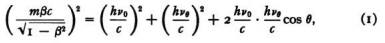
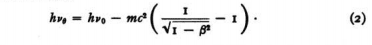
From the above equations, Compton solved for two variables namely $\beta$ the ratio of electron speed to the velocity of light, and for $\nu_{\theta}$, the frequency of the scattered photon. He re-wrote the solution for the second in wavelength form as it is commonly presented (albeit requiring us to replace $2\sin^2 \frac{\theta}{2}$ with $1-\cos\theta$ where $\theta$ is the scattering angle):

It is not quite clear why Compton wrote out the cosine rule with a “+” sign rather than a “-” in Equation 1 but, as noted by PF user Charles Link, Equation 5 above is correct as it stands using the substitution $2{\sin}^2\frac{\theta}{2}=1-\cos\theta$.

A New Angle

We are  going to follow a similar path to that of Compton in terms of solving for 2 variables. But our selection of variables to be solved will be a little different in light of the major output parameters of a Compton scattering event – namely the kinetic energy attained by the electron (which corresponds to the change in photon energy) , the angle of deviation of the incident photon (ie scattering angle) and finally the recoil angle of the electron. We begin by introducing an additional angle to the scattering equations by making the following simple substitution: $$sin\delta=\beta=\frac{v_e}{c},$$ with $\beta$ as defined above from Compton’s paper. It will be immediately apparent that the electron’s Lorentz factor $\gamma=\frac{1}{\sqrt{(1-\beta^2)}}$ can then be written very simply as: $$\gamma=\sec\delta.$$ Electron momentum can  be conveniently represented as: $$p_e=m_ec\tan\delta=\frac{E_0\tan\delta}{c},$$ whilst for kinetic energy we can write: $$T_e=m_ec^2(\sec\delta-1)=E_0(\sec\delta-1),$$ where $E_0=m_ec^2.$

Transforming Compton’s Equations

We can now transform Compton’s equation (1) by multiplying through by $c^2$ and making some additional substitutions: $$E_0=m_ec^2,$$ $$E_1=h\nu_0$$and$$E_2=h\nu_{\theta}.$$Equation 1 can then be written as follows: $${E_0}^2\tan^2\delta=E_1^2+E_2^2-2E_1E_2\cos\theta.$$ Per recommendation of PF User Vela, we complete the square on the right hand side: $${E_0}^2\tan^2\delta={\Delta E}^2+2E_1E_2(1-\cos\theta),$$where $\Delta E=E_1-E_2.$

Equation 2 can be similarly transformed: $$E_0(\sec\delta-1)=E_1-E_2$$ $$⇒E_0\sec\delta=E_0+\Delta E,$$ whereby we can square on both sides leading to: $${E_0}^2{\sec}^2\delta={E_0}^2+{\Delta E}^2 + 2E_0\Delta E.$$Subtracting Equation 1 and employing the identity ${\sec}^2\delta-{\tan}^2\delta=1$ leads to: $${E_0}^2={E_0}^2+2E_0\Delta E-2E_1E_2(1-\cos\theta)$$ $$⇒E_0\Delta E=E_1E_2(1-\cos\theta)$$ $$⇒{E_0}^2(\sec\delta-1)=E_1E_2(1-\cos\theta), $$ or $$\frac{{E_0}^2}{E_1E_2}=\frac{1-\cos\theta}{\sec\delta-1}.$$

Where appropriate in the above equation, we can substitute either $E_2=E_1-\Delta E =E_1-E_0(\sec\delta-1)$ or $E_1=E_2+\Delta E =E_2+E_0(\sec\delta-1)$. So given the scattering angle, we can calculate the change in photon energy, or conversely given the change in photon energy, we can calculate the scattering angle. We appear to have ‘collapsed’ a pair of simultaneous equations into a single equation relating the change of photon energy to scattering angle. However it should be noted that Compton’s Equation 2 is not really the second in a pair – it just supplies us with $\Delta E$ for use in the equation above. In principle, however, we can easily determine Compton’s $\beta$ parameter from the sine of angle $\delta$ if required.

Vector Diagram: x-axis is the direction of motion of incident photon.

Using the representation of electron momentum obtained above, we can also redraw Compton’s vector diagram and resolve vectors horizontally and vertically:

 

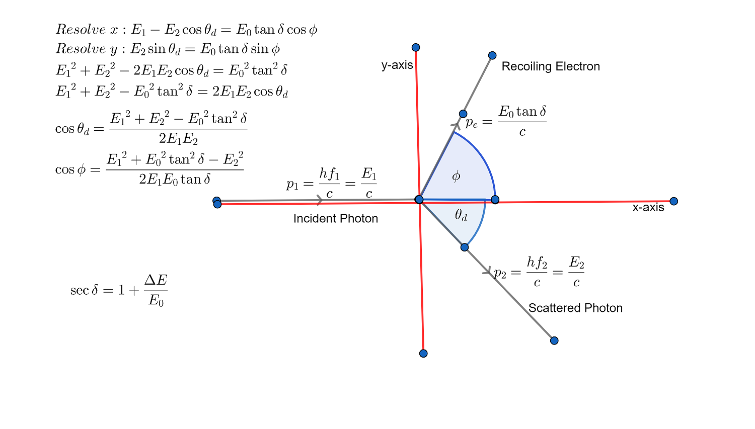
From the vertical (y) resolution, we can immediately write down an expression enabling us to determine the electron recoil angle $\phi$: $$ \sin\phi=\frac{E_2\sin\theta_d}{E_0\tan\delta}$$

Worked Example

Note: The various worked examples in this article are largely the same as in the previous but – for the most part – we employ different methods of solution illustrating the equations developed herein.

From Libre Texts, the problem is to determine the kinetic energy and recoil angle of an electron following the scattering of an 800 keV photon. The scattered photon has energy 650 keV.

Solution

The first part of  the problem is straightforward – kinetic energy of the electron will be the difference in energy of incident and scattered photons ie 800 keV – 650 keV = 150 keV. For part 2 we need to determine angles $\delta$ and $\theta_d$ so that we can use the expression (for electron recoil angle) developed above:

$$\sec\delta=1+\frac{\Delta E}{E_0}=1+\frac{150 \; keV}{512 \; keV}⇒\delta=39.339^{\circ}$$

$$\cos\theta_d=1-\frac{E_0\Delta E}{E_1E_2}=1-\frac{512 \;keV \times 150 \;keV}{800 \;keV\times 650 \;keV}⇒\theta_d=31.536^{\circ}$$

$$ \sin\phi=\frac{E_2\sin\theta_d}{E_0\tan\delta}=\frac{650\sin 31.536^{\circ}\;keV}{512\tan 39.339^{\circ}\;keV}⇒\phi=54.111^{\circ}$$

Alternatively we can simply divide the x and y resolved vector equations to obtain:

$$\tan\phi=\frac{E_2\sin\theta_d}{E_1-E_2\cos\theta_d}=\frac{650\sin 31.536^{\circ}\;keV}{800\;keV  – 650\cos 31.536^{\circ}\;keV}⇒\phi=54.111^{\circ}$$

Additional Note

The following is an important manipulation of the above equation for $\tan\phi$ since – by eliminating $E_2$ – it enables us to deal with problems in which we only have angular information on the recoiling electron and scattered photon:

Starting with $$\tan\phi=\frac{E_2\sin\theta_d}{E_1-E_2\cos\theta_d}, $$ we begin by adding and subtracting $E_2$ in the denominator: $$\tan\phi=\frac{E_2\sin\theta_d}{E_1-E_2+E_2-E_2\cos\theta_d}=\frac{E_2\sin\theta_d}{\Delta E+E_2(1-\cos\theta_d)}$$ Next we use the substitution $1-\cos\theta_d=\frac{E_0\Delta E}{E_1E_2}$ and multiply numerator and denominator by $E_0E_1$: $$\tan\phi=\frac{E_0E_1E_2\sin\theta_d}{E_1E_0\Delta E+{E_0}^2\Delta E}=\frac{E_0E_1E_2\sin\theta_d}{E_0\Delta E(E_1+E_0)}.$$Noting that $\frac{E_1E_2}{E_0\Delta E}=\frac{1}{1-\cos\theta}$, we can simplify: $$\tan\phi=\frac{E_0\sin\theta_d}{(E_0+E_1)(1-\cos\theta_d)}=\frac{E_0}{E_0+E_1}\cot(\textstyle\frac{\theta_d}{2})$$

Vector Diagram: x-axis is the direction of motion of the recoiling electron

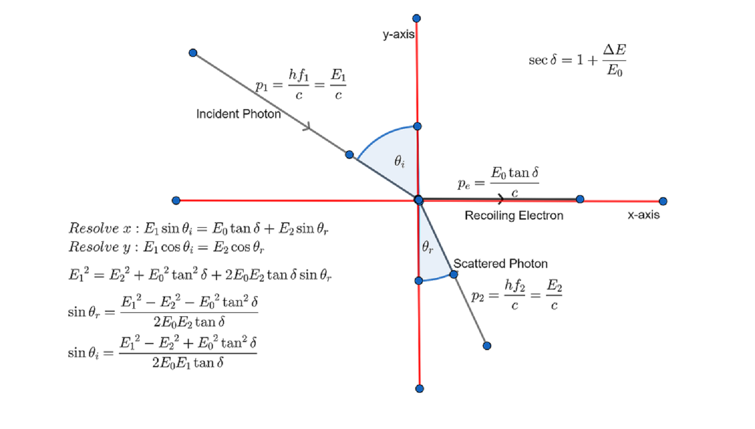
From the resolution of y-components above, it is worth noting that we have a Snell’s law type relationship albeit involving cosines rather than sines of the incident and refracted angles: $$\cos\theta_r=\frac{E_1}{E_2}\cos\theta_i=\frac{f_1}{f_2}\cos\theta_i$$In ‘conventional’ refraction, the refractive index is a ratio of velocities whereas here it is a ratio of energies or frequencies.

Angle Relationships

If we examine the geometry of the two vector diagrams discussed above, we can relate the respective angles as follows:

$$\theta_d=\theta_i-\theta_r,$$  $$\phi=90-\theta_i$$and$$\theta_d+\phi=90-\theta_r.$$

Worked Example

A problem that appeared in one of the PF homework forums was (essentially) to show that if the post-impact trajectories of scattered photon and recoiling electron are at right angles to each other, then the scattered photon has energy equal to the rest mass of the electron.

Solution

The applicable condition for this problem is that $\theta_r=\sin\theta_r=0$. So, from the expression given for $\sin\theta_r$ in the diagram above,  our task is to solve the equation: $${E_1}^2-{E_2}^2-{E_0}^2{\tan}^2\delta=0.$$ The last term in the expression on the left hand side (square of electron momentum$\times c^2$) can be re-written as follows: $$ {E_0}^2{\tan}^2\delta={E_0}^2({\sec}^2\delta-1)={E_0}^2[(\sec\delta-1)^2+2\sec\delta-2)]={\Delta E}^2+2E_0 \Delta E$$. Substituting in the original equation gives: $${E_1}^2-{E_2}^2-{\Delta E}^2-2E_0 \Delta E=0,$$ $$2E_1E_2-2{E_2}^2-2E_0 \Delta E=0,$$ $$E_2\Delta E-E_0\Delta E=0,$$ $$\Delta E(E_2-E_0)=0.$$Hence $E_2=E_0$ as required.

The analysis above has a serendipitous by-product which is the simplification of the expression for $\sin\theta_r$: $$\sin\theta_r=\frac{(E_2-E_0)E_0(\sec\delta-1)}{E_0E_2\tan \delta}=\frac{E_2-E_0}{E_2}\tan(\textstyle\frac{\delta}{2}).$$From this form of the equation for $\sin\theta_r$ it is immediately apparent that the numerator will be zero if $E_2=E_0$. Furthermore if we use this equation to determine $\theta_r$, we can again divide x and y resolved vector equations to find $\cot\theta_i$: $$\cot\theta_i=\tan\phi=\frac{E_2\cos\theta_r}{E_0\tan\delta+E_2\sin\theta_r}$$

Time-Reversal Invariant

From Encyclopaedia Britannica

Time reversal, in physics, mathematical operation of replacing the expression for time with its negative in formulas or equations so that they describe an event in which time runs backward or all the motions are reversed. A resultant formula or equation that remains unchanged by this operation is said to be time-reversal invariant, which implies that the same laws of physics apply equally well in both situations, that the second event is indistinguishable from the original, and that the flow of time does not have any naturally preferred direction in the case of fundamental interactions. A motion picture of two billiard balls colliding, for example, can be run forward or backward with no clue to the proper time direction of the event.

The consequence of Compton scattering being ‘time-reversal invariant’ is that if we imagine a video reversal of a Compton scattering event, it should be a valid physical process. The ‘time reversed’ version of a Compton scattering event involving stationary electrons will be a photon or photon stream interacting with electron(s) moving at a specific angle (measured from the direction of motion of the photons) leading to the electrons coming to a standstill and the photon(s) picking up the energy and being deflected through the same scattering angle (reverse Compton scattering) as in the ‘forward time’ scattering event. As an example, let us ‘reverse engineer’ the Libre Texts problem.

Worked Example

A beam of gamma-ray photons with energy $650\;keV$ crosses the path of (collides with) a beam of electrons and is deflected through an angle of $31.54^{\circ}$. Determine the kinetic energy of the electrons in the electron beam and the angle at which the two beams cross if the electrons are stopped.

Solution

We have been given the angle of deflection and are asked to determine $\Delta E$ which in this case will be the pre-collision kinetic energy of the stopped electrons. $$\Delta E=\frac{{E_2}^2(1-\cos\theta_d)}{E_0-E_2(1-cos\theta_d)}=\frac{{650}^2(1-\cos(31.54^{\circ}))\;{keV}^2}{512 \;keV – 650(1-cos(31.54^{\circ}))\;keV}=150.04\;keV$$

Next we determine angle $\delta$ by using the relationship $E_0(\sec\delta-1)=\Delta E$:

$$\sec\delta=1+\frac{\Delta E}{E_0}=1+\frac{150.04 \;keV}{512\;keV}⇒\delta=39.34^{\circ}$$

To calculate electron angle we can now use the formula:

$$\sin\phi=\frac{E_2\sin\theta_d}{E_0\tan\delta}=\frac{650\sin(31.54^{\circ})\;keV}{512\tan(39.34^{\circ})\;keV}⇒\phi=54.12^{\circ}.$$

 

The beams cross at an angle of $\theta+\phi=31.54^{\circ}+54.12^{\circ}=85.66^{\circ}.$

Alternatively we can use our equation for determining $\theta_r$:

$$\sin\theta_r=\frac{E_2-E_0}{E_2}\tan({\textstyle\frac{\delta}{2})}=\frac{650\;keV-512\;keV}{650\;keV}\tan({\textstyle\frac{39.34}{2}})⇒\theta_r\approx4.35^{\circ}$$

$$\theta_d+\phi=90^{\circ}-\theta_r \approx 85.65^{\circ}$$

Electron ‘Stopper’

We have previously shown that if the post collision trajectories of electron and scattered photons are at right angles, the energy of the scattered photons will be equal to the rest mass of the electron. Conversely if we were to fire a beam of gamma ray photons having energy equal to electron rest mass $(\approx 512\;keV)$ at right angles to a beam of electrons, we would expect to ‘stop’ the electrons and transfer their energy to the beam of gamma ray photons which would deflect through a certain angle depending on the original kinetic energy of the electrons. Given:$$E_2(1-\cos\theta_d)=\frac{{E_0}^2(\sec\delta-1)}{E_2+E_0(\sec\delta-1)},$$ substitute $E_2=E_0$ obtaining $$1-cos\theta_d=\frac{\sec\delta-1}{\sec\delta}=1-\cos\delta.$$Hence $\cos\theta_d=\cos\delta$ and $$\sin\theta_d=\sin\delta=\frac{v}{c}.$$For v<<c, angle of deflection would be directly proportional to electron velocity since $\sin\theta_d\approx\theta_d$.

An interesting property of this particular situation is that we can write: $$\frac{E_1}{E_2}=\frac{E_2+\Delta E}{E_2}=\frac{E_0+(\gamma-1)E_0}{E_0}=\gamma$$ This corresponds to the ratio of frequencies in the “transverse Doppler effect” for a light-emitting source moving at right angles to the line between source and observer at the point of closest approach.

The Caveat to “Reverse-time” Calculations

PF user mfb points out that although the above calculations do yield plausible outcomes to the described scattering events, they are not the only possible outcomes:

Consider the situation of a photon and an electron (both moving) in the center of mass frame. It’s always a head-on collision and photon and electron will fly away again with the same energy as before but in a random direction. Only one of these directions can correspond to an electron at rest in the lab frame.

If it is physically not possible to  ‘orchestrate’ the scattering such that the ‘electron stopping’ event can be isolated or enhanced compared to other outcomes, then one can only conclude that the above calculations are ‘of academic interest’ only. However, there is room for optimism in light of the research mentioned under the “Related Research” heading below.

Related Research

The concept of ‘stopping’ electrons with photon energy is not new. See for example the following article:

https://www.forbes.com/sites/meriameberboucha/2018/02/11/scientists-prove-that-light-can-stop-electrons/#cc464f76b421

The “reverse” Compton scattering discussed in this article may not be possible at present because gamma-ray lasers are not (yet) available – the highest energy levels of laser light are currently in the UV range. All the same, there has certainly been no shortage of research efforts directed at trying to produce such a device:

https://en.wikipedia.org/wiki/Gamma-ray_laser#References

A very recent research effort aims to produce Gamma rays through the mutual annihilation of electrons and positrons – one would guess this would produce exactly the photon energy $(\approx512\;keV)$  required for “electron stopping” as described in this article. Roll on the gamma-ray laser!

https://phys.org/news/2019-12-gamma-ray-laser-closer-reality.html

Summary and Conclusions

In this article, we have ‘dissected’ the important phenomenon of Compton Scattering by examining it through the ‘lens’ of resolved vector diagrams. To do this, we introduced what might be termed the “energy angle” $\delta$ where $\sin\delta=\beta=\frac{v_e}{c}$ so that important parameters such as the electron’s momentum and kinetic energy could be conveniently represented by expressions relating to this angle.

In the first vector diagram, we resolved parallel and perpendicular to the direction of motion of the incident photon and in the second parallel and perpendicular to the direction of motion of the recoiling electron. Angles in the two diagrams are related by simple geometry. A number of different expressions for electron recoil angle were derived and  ‘tested’ in various worked examples.

We furthermore noted that Compton Scattering is “reverse time-invariant” and examined some consequences of this property.

List of Formulae

$$\sin\delta=\beta=\frac{v_e}{c};\sec\delta=1+\frac{\Delta E}{E_0}$$

$$1-\cos\theta_d=\frac{E_0\Delta E}{E_1E_2}$$

$$\tan\phi=\frac{E_2\cos\theta_r}{E_0\tan\delta+E_2\sin\theta_r}=\frac{E_2\sin\theta_d}{E_1-E_2\cos\theta_d}=\frac{E_0}{E_0+E_1}\cot(\textstyle\frac{\theta_d}{2})$$

$$\sin\theta_r=\frac{E_2-E_0}{E_2}\tan(\textstyle\frac{\delta}{2}).$$

Acknowledgements

The Wolfram Alpha computational engine has been employed to good effect in determining some useful (but perhaps obscure) trigonometrical identities involving half angles. The vector diagrams were drawn up using another online site called GeoGebra.

I requested PF users vanhees71 and mfb to cast an eye over this article with particular reference to the time-reversal aspects. The former responded as follows to the specific question as to whether Compton Scattering is indeed a “time-reversal invariant” process:

In this case of Compton scattering of course also the entire dynamics is time-reversal invariant because the electromagnetic interaction is time-reversal invariant (as are all fundamental interactions in the standard model except the weak interaction).

PF user mfb provided the above ‘caveat’ to the reverse-time scattering events considered in this article. He also advised that ‘state of art’ lasers do have energies above the UV range:

Free electron lasers can produce tens of keV in their radiation (~30 keV for the European XFEL) – not 511 keV, but closer to that than the UV range you mention.

Both reviewers indicate that Compton Scattering is best analyzed using 4-vectors:

The kinematics is also quite complicated compared to a covariant treatment.

The author would like to expressly thank both reviewers and acknowledges that the mathematics of 4-vectors is outside the scope of a more limited engineering Maths background.

References

 

[1]	Arthur H. Compton. compton.pdf. https://history.aip.org/history/exhibits/gap/PDF/compton.pdf. (Accessed on 08/05/2020). [ bib ]
[2]	Paul D’Alessandris. 4.2: Compton scattering – physics libretexts.https://phys.libretexts.org/Bookshelves/Modern_Physics/Book%3A_Spiral_Modern_Physics_(D’Alessandris)/4%3A_The_Photon/4.2%3A_Compton_Scattering. (Accessed on 08/05/2020). [ bib ]
[3]	Encyclopedia Britannica. Time-reversal invariance | physics | Britannica. https://www.britannica.com/science/time-reversal-invariance. (Accessed on 08/05/2020). [ bib ]
[4]	Wikipedia Contributors. Relativistic Doppler effect – wikipedia.https://en.wikipedia.org/wiki/Relativistic_Doppler_effect#Transverse_Doppler_effect. (Accessed on 08/07/2020). [ bib ]
[5]	Meriame Berboucha. Scientists prove that light can stop electrons.https://www.forbes.com/sites/meriameberboucha/2018/02/11/scientists-prove-that-light-can-stop-electrons/#7d17c5356b42. (Accessed on 08/05/2020). [ bib ]
[6]	Iqbal Pittalwala. Gamma-ray laser moves a step closer to reality.https://phys.org/news/2019-12-gamma-ray-laser-closer-reality.html. (Accessed on 08/05/2020). [ bib ]

---

Read my next article: https://www.physicsforums.com/insights/equations-of-motion-revisited/

Comment Thread