Bases for Tangent Spaces and Subspaces - McInerney Theorem 3.3.14

In summary: The theorem states that there are two sets of basis vectors, which are chosen along the direction of differentiation. The vectors are linearly independent because their dot product is always zero.
  • #1
Math Amateur
Gold Member
MHB
3,990
48
TL;DR Summary
The thread concerns a basis for a tangent space ...
I am reading Andrew McInerney's book: First Steps in Differential Geometry: Riemannian, Contact, Symplectic ... and I am focused on Chapter 3: Advanced Calculus ... and in particular on Section 3.3: Geometric Sets and Subspaces of ##T_p ( \mathbb{R}^n )## ... ...

I need help with an aspect of the proof of Theorem 3.3.14 ... ...

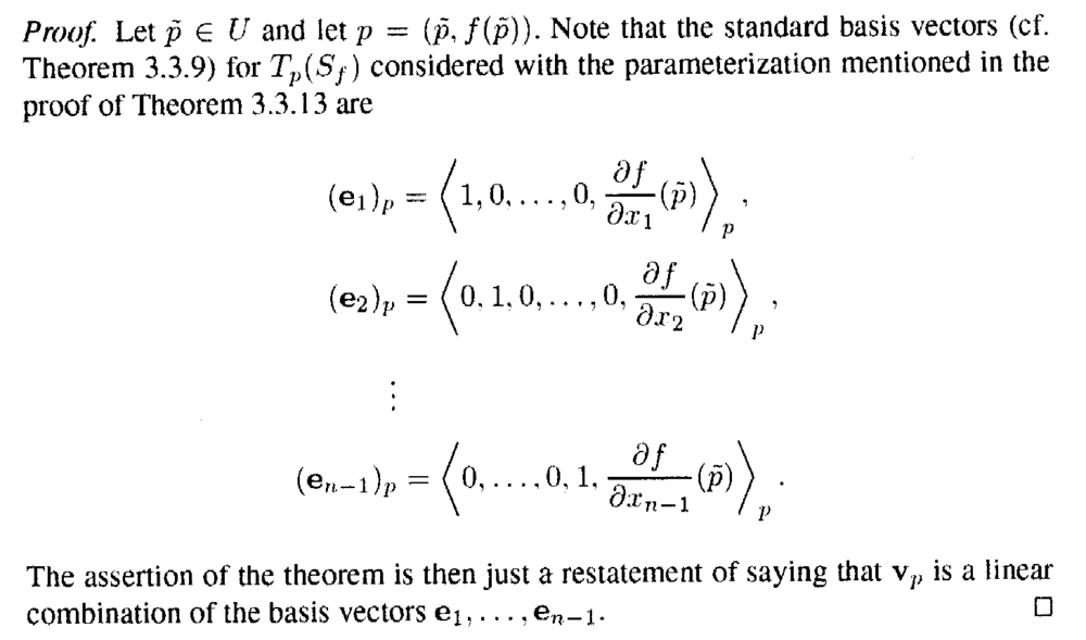
Theorem 3.3.14 reads as follows:
McInerney - 1 - Theorem 3.3.14 ... ... Page 1 ... .png

McInerney - 2 - Theorem 3.3.14 ... ... Page 2 ... .png


Can someone please explain/demonstrate explicitly why/how ##(e_1)_p, (e_2)_p, \ ... \ ... \ , (e_{n-1} )_p## are the standard basis vectors for ##T_p( S_f )## ...Help will be much appreciated ... ...

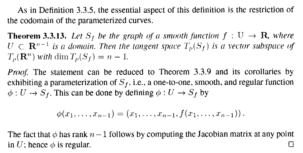
Peter==================================================================================================================The above post mentions Theorem 3.3.13 so I am providing text of the theorem together with a relevant definition ... as follows:
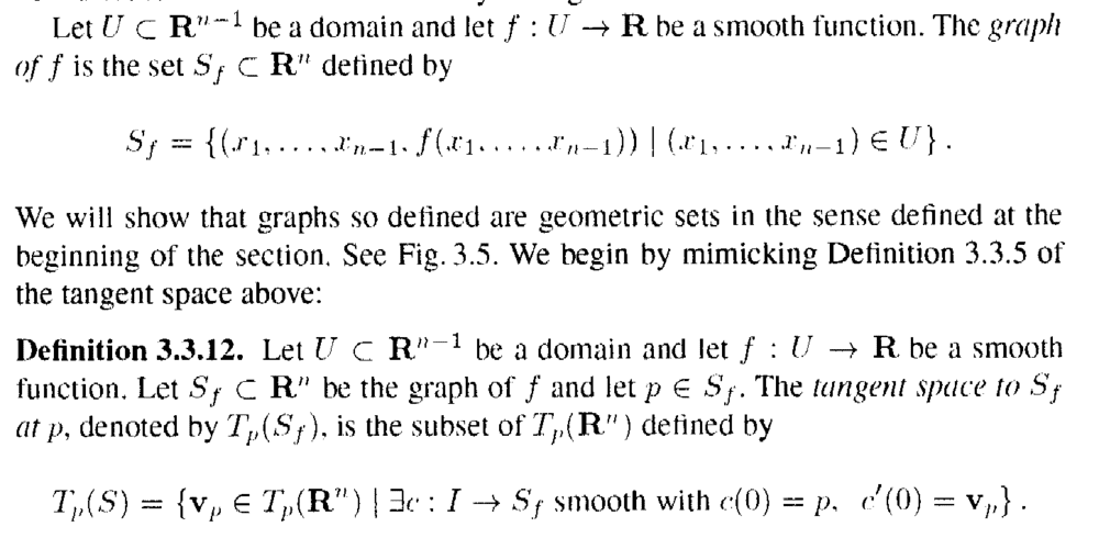
McInerney - Defn 3.3.12 & Theorem 3.3.13 ... ... Page 1 ... .png

McInerney - 2 - Defn 3.3.12 & Theorem 3.3.13 ... ... Page 2 ... .png

Hope that helps readers follow the post ...

Peter
 
Physics news on Phys.org
  • #2
Try to imagine the case ##n=2##. Then we would have some surface in three dimensional space as the graph of the function, e.g. https://www.wolframalpha.com/input/?i=f(x,y)=-x^2-0.3+xy+5.

The tangent space is then a (hyper-)plane ##H## touching the graph at a certain point ##p##. (It may also intersect the graph elsewhere, but this is irrelevant. Differentiation and tangents are a local phenomenon and we are only interested in what happens around ##p##.) Next which coordinates of ##H## can we choose? We take ##p## as origin of our coordinate system. We will consider the tangent space as a linear space with coordinates in its own, and not an affine space ##p+H## which we get, if we will take the 'outer' coordinates of ##\mathbb{R}^3##. However, we want to stay within ##T_p(f)## and there are only two basis vectors and ##p## is their origin. But which ones to take? From ##p## we can go in any direction. Standard would be, however, to go along the coordinates we differentiated along, that is ##x =x_1## and ##y=x_2##. So the tangent vectors which provide the coordinates along the direction of differentiation are ##(1,0,\frac{\partial f}{\partial {x_1}}) \triangleq (x, \partial_xf) ## and ##(0,1,\frac{\partial f}{\partial {x_2}}) \triangleq (y,\partial_yf)##.

Remember that the tangent vectors are those along any curve ##c## within the graph at the point ##p##. Now we simply have chosen two curves (out of any) in ##x_1## and ##x_2## direction. Two are enough to span ##H##.

The same goes for higher dimensions ##n>2##.
 
  • #3
Thanks fresh_42 for a most helpful post ...

Reflecting on what you have written ...

Peter
 
  • #4
Let ##p = (p_1,...,p_n)## and ##q=(p_1,...,p_{n-1})## its projection on the hyperplane H given by ##x_n=0## (note that means that ##p_n=f(p_1,...,p_{n-1})=f(q)##). You can think of H as the horizontal plane in the 3D case, in which case q is the spot on H that is vertically below p, and that maps to p under function ##f##.

For ##j = 1,...,n-1## let ##b_j(t)=q + t \mathbf e_j##, and then define ##c_j(t) = \bigg(b_j(t),f(b_j(t))\bigg) ##.

Then it is not difficult to show that ##c_j(0)=p## and ##(c_j)'(0) = (\mathbf e_j)_p## so that all the ##(\mathbf e_j)_p## are in the tangent space (by 3.3.12).

We can also show that the vectors ##(\mathbf e_j)_p## are linearly independent. Indeed, I think that may have already been implicitly proved in one of the other threads you posted about this text, about the rank of a Jacobian.

We then use Thm 3.3.13 that tells us the tangent space is a n-1 dimensional subspace. Linear algebra tells us that any set of n-1 linearly independent vectors in a n-1 dimensional space forms a basis for that space, so the n-1 vectors ##(\mathbf e_j)_p## are a basis for the tangent space.

Don't worry about his use of the words 'standard basis vectors'. I think he just means that he will be using them as his default basis for the subspace, not that they have some special property of 'standardness'. Indeed, the vectors do not all have length 1, which is a property often sought in 'standard' bases.

Edited 5:25 pm 20/4/19 to correct an error in the formula for ##c_j(t)##, which then enabled a simplification of the formula.
 
Last edited:
  • #5
Thanks Andrew ...

Thinking through what you have written ...

Peter
 

What is the McInerney Theorem 3.3.14?

The McInerney Theorem 3.3.14 is a mathematical theorem that states that for any smooth manifold M, the tangent space at any point x in M can be decomposed into a direct sum of the tangent space at x and the subspace of vectors that are tangent to the level sets of a given smooth function on M.

What is the significance of the McInerney Theorem 3.3.14?

The McInerney Theorem 3.3.14 is significant because it provides a way to understand and analyze the tangent spaces and subspaces of a smooth manifold. This can be useful in various fields such as differential geometry, physics, and engineering.

How is the McInerney Theorem 3.3.14 related to tangent spaces and subspaces?

The McInerney Theorem 3.3.14 is directly related to tangent spaces and subspaces as it provides a decomposition of the tangent space into the tangent space at a point and the subspace of vectors tangent to the level sets of a given smooth function.

What are some real-world applications of the McInerney Theorem 3.3.14?

The McInerney Theorem 3.3.14 has various real-world applications, such as in the study of differential equations, optimization problems, and geometric modeling. It can also be used in the analysis of physical systems, such as in mechanics and fluid dynamics.

Are there any limitations or exceptions to the McInerney Theorem 3.3.14?

Like any other mathematical theorem, the McInerney Theorem 3.3.14 has its limitations and exceptions. It may not hold for non-smooth manifolds or in certain special cases. Additionally, the theorem may not be applicable in situations where the smooth function used in the decomposition is not well-behaved.

Similar threads

Replies
1
Views
1K
Replies
4
Views
2K
Replies
4
Views
2K
  • Differential Geometry
Replies
12
Views
3K
  • Topology and Analysis
Replies
2
Views
2K
Replies
4
Views
2K
  • Topology and Analysis
Replies
3
Views
1K
Replies
2
Views
1K
Replies
2
Views
1K
Back
Top