Solving 2nd Order ODEs with Euler & Runge-Kutta 4

[Livethefire]

For weeks I've been coding a program to simulate waves on a string. Currently I am working on some numerical methods. Namely Euler and Runge-Kutta. I have Euler working fine as far as I can see for a variety of input waveforms (of course after it runs for a while it goes a bit beserk due to inaccuracies).

I can't for the life of me figure out to implement The RK4 method though. It gets messy. I've searched for the past few weeks, on the internet and every forum I can find to see if I can understand the method better and I can't get my head around it.

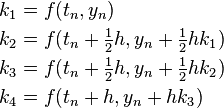
Im using the "standard" equations on Wiki. And the first thing I am really confused about is the f(x, t) function for example.. which is intuitive for the euler method I feel, but whenever there are 4 extra terms, I am lost as to what to do with them.

This is my euler method. A bit chunky I know, but it works.

I Have a string that is broken up into a number of elements, the arrays yold, ynew, vold, vnew and a Hold the position, velocity and acceleration of each element.
This is just the euler routine, I have a much larger piece of code which shows the wave and animates it with a graphics package, and it does what its supposed to.

  int i;
  //Fixed ends, loop runs through 2nd element and 2nd to last element in array
  for(i=1; i<(n-1); i++){
       //calculates the acceleration of each element
      [COLOR="Red"] a[i]=(k/mass_per_n)*((yold[i-1]-yold[i])+(yold[i+1]-yold[i]))[/COLOR]
       //and its velocity with euler
       [B]vnew[i]=vold[i]+a[i]*dt;[/B]
  }
  for(i=1; i<(n-1); i++){
     Then calculates position with euler
    [B] ynew[i]=yold[i]+vold[i]*dt; [/B]     
  }

Where the red shows the differential equation I am going to solve (2nd order ODE). This line is also my acceleration calculation.

And the bold shows my two euler approximations, twice because I am solving a 2nd order ODE.

My problem now is how do I replace these bold statements with the RK4 approximation?
I have another program set up with more arrays but any attempt at RK4 just doesn't work.
Specifically, I am confused abotu how to do it twice, and how do I approximate the function f for k2, k3, and k4?

For the euler method I just multiplied the time step by either velocity or acceleration (see code above).

Thank you for any help or guidance you can give to me on the matter.
Cheers.

 

[rcgldr]

The main advantage of RK4 is speed of computation. If the speed isn't an issue, you can use a predictor-corrector method that iterates more times on each generated data point, and uses small time steps to improve the accuracy. Example of a predictor-corrector method using trapezoidal method:

http://en.wikipedia.org/wiki/Predictor-corrector_method#Euler_trapezoidal_example

Getting back to RK4, k1 is acceleration based on the current data point f(t_n, y_n), k2, k3, k4 are iteration steps to produce 3 intermediate accelerations based on calculated data points (y_guess). h is the time step. If time isn't a factor in determining accelerations, but only position, such as position versus a gravity source, then f(...) is only a function of position (y_n).

In your case, using a(...) to represent your acceleration equation, and vn and yn to represent the array vnold[...] and ynold[...], meaning you have to generate an array of vn's and yn's for each step:

 

[Livethefire]

Thanks for the reply,

Yeah I think I understand what you are saying. Does this not need to be done twice though?

How does, k2, k3, k4 can't really fit into my acceleration equation?
The acceleration is computed by comparing the distances between 3 neighbouring points in the string ( Hookes law approach ). I don't really know where the k's come into it at all?Speed will be an issue late, but right now I want to get the approximation working.

Thanks again for any help.

 

[Filip Larsen]

And the bold shows my two euler approximations, twice because I am solving a 2nd order ODE.

My problem now is how do I replace these bold statements with the RK4 approximation?
I have another program set up with more arrays but any attempt at RK4 just doesn't work.
Specifically, I am confused abotu how to do it twice, and how do I approximate the function f for k2, k3, and k4?

The normal approach would be to turn the second order ODE's (second order derivatives of state position) into a system of first order ODE's (first order derivatives of state position and velocity) and then integrate this. For instance, in the second order ODE

$$\ddot{y} = a\dot{y} + b$$

we can introduce the velocity state $v = \dot{y}$ which inserted gives a system of first order ODEs

$$\begin{array}{l}\dot{y} = v \\ \dot{v} = a v + b\end{array}$$

Solving this system using a Runge-Kutta method, the field is thus a vector field in the state vector $x = (y,v)^T$, i.e.

$$f(x,t) = \dot{x} = \left(\begin{array}{c}\dot{y} \\ \dot{v} \end{array}\right)$$

which also means that the RK4 stage calculations on the state and field are all vector calculations. You can of course choose to inline these vector calculations as (in this case) two calculations involving normal scalars.

 

[rcgldr]

How does, k2, k3, k4 can't really fit into my acceleration equation?

The k's are estimates of acceleration, and are averaged to calculate each new position.

You could just try trapeziodal rule to improve things a bit (you'd need to initialize then use an aold[] and vold[] arrays to save previous accelerations and velocities):

vnew=vold+.5*dt*(aold + a)
ynew=yold+.5*dt*(vold + vnew)

Using corrector iteration requires temp data and another layer of looping. The "j" loop doesn't appear to be doing much, but the values will quickly converge to specific values because the acceleration calculation is being used as feedback in the loop. Although I used 8 loops (... j < 8 ...) in this example, 4 or 6 may be enough. The convergence is to the best trapezoidal approximation though, so the time step needs to remain small to keep everything accurate.

    for(i = 0; i < n; i++){
        ytmp[i] = yold[i];
        vtmp[i] = vold[i];
        atmp[i] = aold[i];
    }

    for(j = 0; j < 8: j++){   // feedback loop, the values will converge
        for(i = 1; i < (n-1); i++){ // new position based on acceleration
            vtmp[i] = vold[i]+.5*dt*(aold[i] + atmp[i]);
            ytmp[i] = yold[i]+.5*dt*(vold[i] + vtmp[i]);
        }
        for(i = 1; i < (n-1); i++){ // new acceleration based on position
            atmp[i]=(k/mass_per_n)*((ytmp[i-1]-ytmp[i])+(ytmp[i+1]-ytmp[i]));
        }
    }

    for(i = 0; i < n; i++){
        ynew[i] = ytmp[i];
        vnew[i] = vtmp[i];
        anew[i] = atmp[i];
    }

 

[Livethefire]

I updated my previous post to replace the k's with v's (velocities) and y's (position).

You could just try trapeziodal rule to improve things a bit:

vnew=vold+1/2*dt(aold + a)
ynew=yold+1/2*dt(vold + vnew)

Ill reiterate what I am trying to achieve for other posters just to be clear.


I wish to model wave on a string. The string is comprised of a number of elements or segments, the position, velocity and acceleration data is held in an array. I.e at x=1, the postion and velcity of that part of the string is held in y[1] and v[1] etc.

Yeah sorry for the editing of my post, kind of confused things.
Yes I understand what the K's actually are, but my equation for acceleration :

a[i]=(k/mass_per_n)*((yold[i-1]-yold[i])+(yold[i+1]-yold[i]))

simply compares the positions between the nearest two elements in the string. So the acceleration of an element is determined by the two nearest beside it.
Your equations:

    y1 = yn
    v2 = vn + .5 * dt * a(y1)

Imply that I can stick in an arbitrary argument to my acceleration function, which as of yet, I cannot ( it is shown above).

Sorry for the confusion, maybe I am missing something obvious.

 

[Filip Larsen]

    vtmp[i] = vold[i]+1/2*dt*(aold[i] + a[i])
    ytmp[i] = yold[i]+1/2*dt*(vold[i] + vtmp[i])
    ...

Be aware, that 1/2*expr in many programming languages are evaluated as involving an integer division and therefore evaluates to 0 (zero). A better form would be (1.0/2)*expr, 0.5*expr or expr/2.0.

 

[rcgldr]

Be aware, that 1/2*expr in many programming languages are evaluated as involving an integer division.

Orignally was just supposed to be comment versus code, I corrected my previous post.

 

[rcgldr]

RK4 code example. I'm assuming that the end points y[0] and y[n-1] never move.

#define y1 yold
#define v1 vold

    y4[0]   = y3[0]   = y2[0]   = y1[0];
    y4[n-1] = y3[n-1] = y2[n-1] = y1[n-1];

    for(i = 1; i < (n-1); i++){ // initial position acceleration
        k1[i] = (k/mass_per_n)*((y1[i-1]-y1[i])+(y1[i+1]-y1[i]));
        v2[i] = vold[i] +      dt*k1[i]; // 1st mid step position
        y2[i] = yold[i] + .5 * dt*v2[i];
    }

    for(i = 1; i < (n-1); i++){ // 1st mid point acceleration
        k2[i] = (k/mass_per_n)*((y2[i-1]-y2[i])+(y2[i+1]-y2[i]));
        v3[i] = vold[i] +      dt*k2[i]; // 2nd mid step position
        y3[i] = yold[i] + .5 * dt*v3[i];
    }

    for(i = 1; i < (n-1); i++){ // 2nd mid point acceleration
        k3[i] = (k/mass_per_n)*((y3[i-1]-y3[i])+(y3[i+1]-y3[i]));
        v4[i] = vold[i] +      dt*k3[i]; // end step position
        y4[i] = yold[i] +      dt*v4[i];
    }

    for(i = 1; i < (n-1); i++){ // end point acceleration
        k4[i] = (k/mass_per_n)*((y4[i-1]-y4[i])+(y4[i+1]-y4[i]));
        aavg = (1./6.)*(k1[i] + 2.*k2[i] + 2.*k3[i] + k4[i]); // avg acc
        vnew[i] = vold[i] + dt*aavg; // new position
        ynew[i] = yold[i] + .5*dt*(vold[i]+vnew[i]);
    }

The corrector iteration code I posted above is a bit simpler to follow, and since it uses calculated acceleration as feedback, it tends to produce better results.

 

[Livethefire]

I think that's what threw me! I didnt have enough position arrays for the midpoints. I've implemented your code and it appears to work fine, although due to my setup Ill need to go through everything with a fine tooth comb- because I've got quite a lot of other processing going on too.

Do keep an eye on this thread, everyone has been of amazing help. And rcgldr thanks again, you have been a life saver, I understand what's going on now!

(side note, your missing ";" at the end of all your statements inside the loops although I am aware that this is just a rough code and I got the jist of what was going on)

I assume all of this can be placed within one loop?

 

[rcgldr]

Note I had to fix the RK4 code example. Since y[i-1], y, and y[i+1] used in acceleration calculation, the y values need to be calculated before being used in the next acceleration calculation loop. The corrector method in post #5 already handles this issue.

I think that's what threw me! I didnt have enough position arrays for the midpoints.

Because position values at [i-1], , and [i+1] are used for each acceleration calculation, they need to be saved.

Ive implemented your code and it appears to work fine

I fixed up a bug in the RK4 code in my previous post (fixed version has aavg in last loop. You might want to try the corrector method from post #5 and compare the results. You can tweak the loop count for (j=0; j<8; j++) to less than 8, 4 may be enough if the function isn't "stiff" (very large change in acceleration versus position).

missing ";"

Wasn't sure if you were coding this in C. I added the semi-colons.

I assume all of this can be placed within one loop?

The accleration calclation uses position values [i-1], , [i+1], so two loops are needed, so position value i+1 can be calculated before it's used in the next acceleration calculation. I had to fix up my RK4 example code to handle this.

 

[Livethefire]

Roughly what I've got is:

main (){

[I]various code setting up arrays etc[/I]

//This function sets up the initial conditions
//And shows it to the screen

initialise_wave(...);

//Loop to cycle through time
for(...t+=dt){

   erase_wave(...);

   //This runge is like what you have in the post before
   runge_kutta(...);

   show_wave(...);

   //loop here using clock() to create pause

   //And this loop resets the arrays
   for(i=1; i<n-1; i++){
      yold=ynew;
   }

}

}

My problem now is that the wave starts off fine, but eventually stops.
For example I have a first sinusoidal mode beginning humped upwards, and it just slows down and stops when it has reached maximum amplitude humped downwards.
I have no idea why.

Also, I thought it was just because the euler method was inaccurate, but for both this and euler, the simulations just goes crazy if I use more than around 10 elements in the string. So what I have now, if I enter in say, 20 elements the string just jerks and goes really spikey off the screen, like a kid scribling on paper.

Whenever I enter the number of elements, that number just defineds the dynamic arrays and the "n" in the loops. Otherwise I thought only the time of the simulation should affect precision. Because If I enter in 20 upwards elements the simulation just instantly goes wrong. This is getting really frustrating now.

Once again thanks for any help. This thread has helped me figure out the RK4 method properly, but evidently I need to go over my programs again or start fresh.

 

[Livethefire]

Anything I try or tweak, it either does what I've mentioned before, or It starts of as half a sine curve and then all the elements slowly go to zero. I.e Starts off fine, but then stays at rest position, it would make me think something isn't right with the acceleration term or something.

I'll Have another proper look at it later.

*EDIT*
This is what I am using at the moment:

    for(i = 1; i < (n-1); i++){ // end point acceleration
        k4[i] = (k/mass_per_n)*((y4[i-1]-y4[i])+(y4[i+1]-y4[i]));
        vnew[i] = vold[i] + (1.0/6.0)*dt*(k1[i] + 2.0*k2[i] + 2.0*k3[i] + k4[i]); // new position
        ynew[i] = yold[i] + 0.5*dt*(vold[i]+vnew[i]);
    }

I figured out that in my main function, I wasnt resetting the velocity arrays aswell.

   for(i=1; i<n-1; i++){
      yold[i]=ynew[i];
      vold[i]=vnew[i];
   }

However, now the simulation runs fine but it loses amplitude? It goes for a few periods and then dies out. Additionally the other problem still persists, whenever I use a large number of elements it goes beserk.

 

[rcgldr]

I would consider switching to the (predictor) corrector code method I showed in post #5, and making dt smaller. dt should probably be 1/1000 of the expected cycle time if not smaller. The corrector code method tends to not accumulate errors if dt is small enough, because of the feedback and convergence. For the corrector code, dt should be 1/2 of the dt value you would use in the RK4 code (to get the equivalent of the mid point values used in RK4).

whenever I use a large number of elements it goes beserk.

What is this acceleration function based on?
k4 = (k/mass_per_n)*((y4[i-1]-y4)+(y4[i+1]-y4));

Are you recalculating mass_per_n if you set n to a higher number?

 

[Livethefire]

Yeah I definitely will, I want to get this RK4 method working first though to compare with my Euler before.

     printf("Please enter number of elements in the string:");
     scanf("%d", &n);
     mass_per_n=pow(10.0/n,2);

or

     printf("Please enter number of elements in the string:");
     scanf("%d", &n);
     mass_per_n=10.0/n;

It doesn't really matter, they both mess up quite quickly. The power just minimises the error initially. And 10.0 is arbitrary. 10Kg for the entire string, split up into elements then mass_per_n is just a division. And k (spring constant) is just 1. The function is a hookes law approximation.

Although keeping a fairly low n, I still don't understand why my wave is dimishing in amplitude. Its a damping free model right now.

 

[rcgldr]

I would consider switching to the (predictor) corrector code method I showed in post #5, and making dt smaller.

Yeah I definitely will, I want to get this RK4 method working first though to compare with my Euler before.

Try making dt smaller to see if that helps.

mass_per_n

It should be mass_per_n=10.0/n (and not (10/n)^2). You might want to change the name to mass_per_e, since it's mass per element.

higher n breaks

How are you assigning the initial position and velocity of each segment?

 

[Livethefire]

I have a function which I call to set up the initial conditions. At the moment its just the fundamental mode sinusoid- sin(pi.x/L). It works fine.

By lowering dt the amplitude diminishes at a rate much less that before. I think dt was my problem. I tried again with 100 elements and it worked fine. These numerical methods do seem very dependant on the initial conditions.. I just assume my code is wrong before I think about the mechanics behind the method! Is the amplitude dimishing a normal thing, or is it just because of the way we accomplished this?

I have dt at 0.1 at the momment, and that works for 100 elements, but at 1000 elements it goes crazy unless I change dt by the same factor (1000 elements works fine with dt at 0.01).

The euler method seems to over estimate and the amplitude gets very large, and that's the way I've seen the RK4 (at a much lesser rate than euler) discribed in textbooks and web resources.

Again thanks for your help. I think I've got the base program working fine. I need to go through it and cut out the bloat though, and I might have a go at an adaptive method.

On a side note, are you a programer, engineer or scientist or none of the above?

 

[rcgldr]

dt = .01 or .001 ... The euler method seems to over estimate and the amplitude gets very large, and that's the way I've seen the RK4 (at a much lesser rate than euler) discribed in textbooks and web resources.

All of these methods are using linear approximations for each period, based on an average acceleration during each period, so dt needs to be small, maybe dt=.0001. The corrector method I showed in post #5 will at least converge to specific values because of the feedback (it predicts the next point, then uses that predicted point as feedback to repredict the next point, converging to a specific point after a few iterations).

I might have a go at an adaptive method.

Adaptive methods are normally used to increase or decrease dt based on current acceleration, in order to speed up the process, but this shouldn't be needed.

The next step up from what you're using now would be a quadratic approximation for each period, but I doubt it ends up being better in terms of accuracy versus compute time.

Are you a programer, engineer or scientist or none of the above?

Programmer, mostly embedded (firmware) and/or multi-tasking oriented work in C with some assembly, with only an occasional math oriented type project.

 

[Livethefire]

Well youve been of great help, I am only a mere physics student still...

I must get to bed however, Ill have a look at it tommorow again.
Thanks

 

[rcgldr]

The method I described in post #5 is known as the two-stage Adams–Moulton method or iterative trapezoidal method.

Wiki articles about instability issue with methods like RK4, and about the method in post #5:

For some differential equations, application of standard methods—such as the Euler method, explicit Runge–Kutta methods, or multistep methods (e.g., Adams–Bashforth methods)—exhibit instability in the solutions

http://en.wikipedia.org/wiki/Numerical_ordinary_differential_equations#Stability_and_stiffness

http://en.wikipedia.org/wiki/Stiff_equation#Motivating_example

http://en.wikipedia.org/wiki/Trapezoidal_method#Adams.E2.80.93Moulton_methods

http://en.wikipedia.org/wiki/Predictor-corrector_method#Euler_trapezoidal_example

I created an example excel spreadsheet demonstrating the method in post #5 for the same equation shown in the wiki article about stiff equations.

y' = -15 y (which can be directly integrated: y = e^-15t)

for t = 0 to 1, showing the actual value, numerically integrated value, and the error value (difference). This is a "stiff" equation, that can be problematic with some numerical integration methods. In this case, the error value decreases in magnitude as the expected answer (e^-15 = 3.059 x 10 ^-7) decreases in magnitude.

http://rcgldr.net/misc/numerical_integration.zip