Sum of many random signals

[roam]

TL;DR Summary

Empirically we know that if we add $N$ signals with independent random phases and amplitudes, the shape of the sum flattens out as $N$ tends to infinity. How can this effect be formally demonstrated?

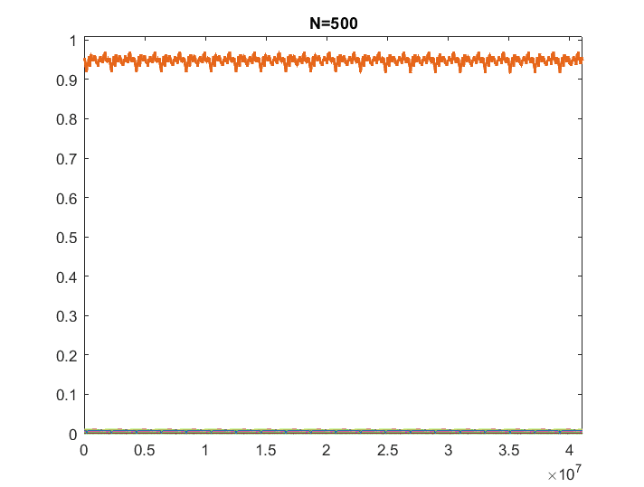
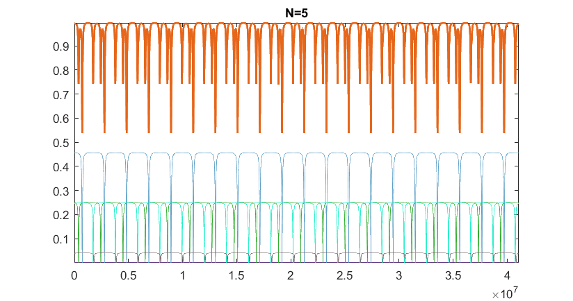
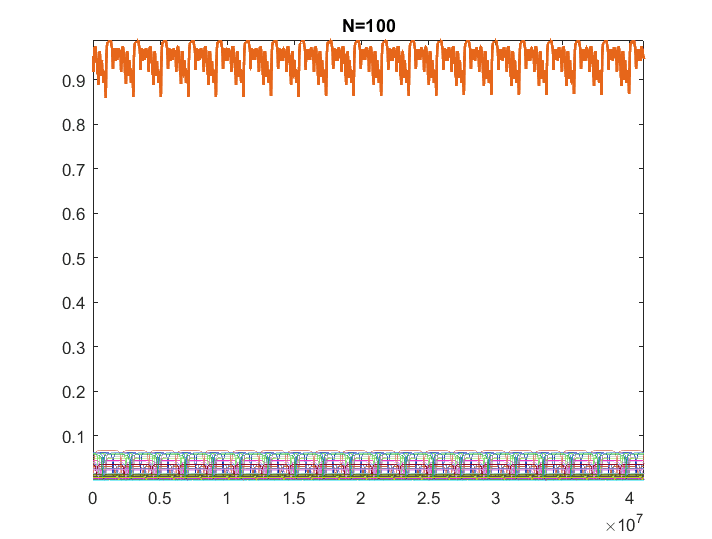
For instance, here is an example from my own simulations where all underlying signals follow the same analytical law, but they have random phases and amplitudes (such that the sum of the set is 1). The thick line represents the sum:

Clearly, the sum tends to progressively get flatter as $N \to \infty$. Is there a formal mathematical way to show/argue that as the number of underlying components increases, the sum must tend to a flat line?

 

[Svein]

Well, first of all the sum of the amplitudes must be finite.

 

[RPinPA]

Summary: Empirically we know that if we add $N$ signals with independent random phases and amplitudes, the shape of the sum flattens out as $N$ tends to infinity. How can this effect be formally demonstrated?

If I understand the question, the answer lies in the Law of Large Numbers, as you are in effect at each time sample looking at the mean of a large number of independent (identically distributed?) random variables.

For instance, here is an example from my own simulations where all underlying signals follow the same analytical law, but they have random phases and amplitudes (such that the sum of the set is 1).

I don't quite understand this description. It looks like all the signals are periodic, is that right? I'm guessing the phases are uniform on $[0, 2\pi]$. How are the amplitudes distributed? Do they all have the same frequency?

 

[roam]

If I understand the question, the answer lies in the Law of Large Numbers, as you are in effect at each time sample looking at the mean of a large number of independent (identically distributed?) random variables.

Hi @RPinPA

Do you know how the Law of Large Numbers might be applicable to this situation? Does the law say that the sum of all those independent random values must approach a specific value?

I don't quite understand this description. It looks like all the signals are periodic, is that right? I'm guessing the phases are uniform on $[0, 2\pi]$. How are the amplitudes distributed? Do they all have the same frequency?

Yes, all the individual signals are periodic. But the periods are slightly differ from each other. The number that determines the phases/periods of the individual curves is sampled from a uniform distribution. The amplitudes were sampled from something similar to an exponential distribution (the values can differ considerably).

I think it is the randomness of the phases which is responsible for the effect, because it causes the curves to overlap in different ways. As $N$ increases, the modulation depth (the magnitude of variation) of the signal also tends to decrease. Is it the Law of Large Numbers that predicts the effect?

Well, first of all the sum of the amplitudes must be finite.

But it is finite. They all add up to a maximum amplitude of 1.

 

[Baluncore]

But it is finite. They all add up to a maximum amplitude of 1.

... they have random phases and amplitudes (such that the sum of the set is 1).

It will depend on how you define the signals. If the n signals are sinewaves, all with identical amplitude fixed at 1/n, but with different frequencies and different initial phases, then the combined amplitudes will form continuously changing sums and differences as the phase of all the different frequency signals slide in and out of phase. Since you are summing energy you must consider the RMS value of the sum of all signal amplitudes.

The frequency spectrum will be orderly, it will show n peaks at n different frequencies, each with the same 1/n amplitude.

 

[RPinPA]

If I understand the question, the answer lies in the Law of Large Numbers, as you are in effect at each time sample looking at the mean of a large number of independent (identically distributed?) random variables.

Do you know how the Law of Large Numbers might be applicable to this situation? Does the law say that the sum of all those independent random values must approach a specific value?

If you can make the case that at each time $t$ you are taking the average of $n$ samples drawn independently from the same distribution, then that average will tend toward the mean of that population distribution as $n \rightarrow \infty$. Since it's the same distribution at each $t$, then all the points will be converging toward the same mean.

You haven't described the procedure yet enough for me to model what that distribution is, but from what you've described so far it does sound like such a model applies.

 

[roam]

If you can make the case that at each time $t$ you are taking the average of $n$ samples drawn independently from the same distribution, then that average will tend toward the mean of that population distribution as $n \rightarrow \infty$. Since it's the same distribution at each $t$, then all the points will be converging toward the same mean.

Hi @RPinPA

So, how do we explain why the mean of the population at all different points tend to a similar value as $n \to \infty$? Is that just something we know a priori from the Law of Large Numbers?

I am looking for a rigorous explanation of why the sum curve gets flatter. Intuitively I think as $n \to \infty$, we have more probability that the maxima of one curve coincides and cancels out the trough of another curve. This decreases the fluctuation depth of the sum and the curve appears flatter.

You haven't described the procedure yet enough for me to model what that distribution is, but from what you've described so far it does sound like such a model applies.

The individual curves are generated using the formula:

$$A.\frac{a^{2}+b^{2}-2ab\cos\varphi}{1+b^{2}a^{2}-2ab\cos\varphi},$$

where the constants are equal to $a=b=0.95$; the random amplitude $A$ is sampled from an exponential distribution (such that the sum of all $A$s is $1$); the random phase term $\varphi$ is taken from a uniform distribution.

 

[RPinPA]

Hi @RPinPA
The individual curves are generated using the formula:

$$A.\frac{a^{2}+b^{2}-2ab\cos\varphi}{1+b^{2}a^{2}-2ab\cos\varphi},$$

where the constants are equal to $a=b=0.95$; the random amplitude $A$ is sampled from an exponential distribution (such that the sum of all $A$s is $1$); the random phase term $\varphi$ is taken from a uniform distribution.

That's a single numerical value for any particular draw of $A$ and $\varphi$. Where does the periodicity come in? What is the horizontal axis?

How can you simultaneously draw $n$ numbers independently from an exponential distribution but make sure the sum of the $A$s is 1? Do you mean that after you draw the values you normalize them?

 

[Marco Aquino]

Clearly, the sum tends to progressively get flatter as N→∞. Is there a formal mathematical way to show/argue that as the number of underlying components increases, the sum must tend to a flat line?If “clearly” is your is your definition of (no other way) than you won’t figure out the best way known (presently).
The sum may not flat line but represent itself to be smaller in your perception. Because our limiting factor is time. It will eventually be greater in value and then lesser in value if time persists.
Presenting it in a math equation?
N=(absolute value)+V1
V1>(sumV2)/T0.9

Hmmm.. I got to find a better way to explain this.

 

[roam]

That's a single numerical value for any particular draw of $A$ and $\varphi$. Where does the periodicity come in? What is the horizontal axis?

The function that I am plotting is known as the "Airy function" which gives the output of a Fabry-Perot etalon. The dips occur whenever $\varphi=2\pi q$, for $q$ being an integer. The period is known as the "free spectral range". The horizontal axis is the frequency $\nu$ which is proportional to the phase term $\varphi$:

$$\nu=\frac{\varphi.c}{2\pi L}.$$

Here $L, c$ are physical constants that signify the length of the etalon and the speed of light.

But the effect is not specific to this function. If you choose other functions and randomly overlap them, the sum of the set tends to get flatter as $N$ increases. The depth of the dips decreases. Why?

How can you simultaneously draw $n$ numbers independently from an exponential distribution but make sure the sum of the $A$s is 1? Do you mean that after you draw the values you normalize them?

Yes, I normalize them later.

 

[roam]

Hi @RPinPA

Do you think it is possible to argue that the result is a consequence of the Central Limit Theorem?

 

[Stephen Tashi]

Hi @RPinPA

Do you think it is possible to argue that the result is a consequence of the Central Limit Theorem?

https://www.physicsforums.com/threads/central-limit-theorem-and-fitting-data.970962/#post-6177142

 

[roam]

https://www.physicsforums.com/threads/central-limit-theorem-and-fitting-data.970962/#post-6177142

But this is a different problem. If we add up a large number of curves with random phases (this could be any function; even sine waves), the sum tends to flatten out. Is this in consequence of the Law of Large Numbers, CLT, or a different law? There has to be a rigorous explanation of this simple effect in statistics.

 

[Stephen Tashi]

Let $f$ be a integrable periodic function with period $L$. One definition of "the mean value of $f$" is $\mu_f = \frac{1}{L} \int_0^L f(x) dx$.

Let $U$ be a uniformly distributed random variable defined on $[0,L]$ and let $x_0$ be an number in $[0,L]$. Define the random variable $X_0$ by $X_0 = f(x_0 - U)$.

Show the expected value of $X_0$ is $E(X_0) = \mu_f$.

The central limit theorem is relevant to the mean value of the sum of $N$ independent realizations of $X_0$.

 

[roam]

If I understood correctly, you are suggesting that as N increases, the value for each variable converges to the expected value, which is the mean value that the underlying function takes. This is basically a definition of the (strong) Law of Large Numbers.

The central limit theorem is relevant to the mean value of the sum of $N$ independent realizations of $X_0$.

The central limit theorem simply tells us that the standard deviation associated with the mean value of the sum gets smaller as $N \to \infty$. As you emphasized earlier, it doesn't tell us anything directly about the actual value of the mean.

As it was mentioned in the other thread, I empirically found that the actual value of the mean varies according to $\mu_f \approx 1/\sqrt{N}$. But we couldn't find a rigorous explanation that connects this effect to the CLT.

Let $U$ be a uniformly distributed random variable defined on $[0,L]$ and let $x_0$ be an number in $[0,L]$. Define the random variable $X_0$ by $X_0 = f(x_0 - U)$.

Could you please explain what would be the significance of $U$? Does it represent the random phase of each underlying curve?

 

[Stephen Tashi]

If I understood correctly, you are suggesting that as N increases, the value for each variable converges to the expected value, which is the mean value that the underlying function takes. This is basically a definition of the (strong) Law of Large Numbers.

Yes, that is correct - if we use the definition of "converges" appropriate to probability theory. This definition is different than the definition of "converges" used in elementary calculus.

Could you please explain what would be the significance of $U$? Does it represent the random phase of each underlying curve?

Yes, one realization of the random variable $U$ is used to determine the phase of one curve.

As it was mentioned in the other thread, I empirically found that the actual value of the mean varies according to $\mu_f \approx 1/\sqrt{N}$. But we couldn't find a rigorous explanation that connects this effect to the CLT.

As mentioned before, you aren't using precise language. You want to talk about functions. Functions aren't single numbers. The realization of a random function is more than one single random number. So the phrase "the mean" is ambiguous. As mentioned above, there is a standard definition for the mean of a periodic function, but I don't think this is the mean that you want to consider.

The central limit theorem simply tells us that the standard deviation associated with the mean value of the sum gets smaller as $N \to \infty$. As you emphasized earlier, it doesn't tell us anything directly about the actual value of the mean.

Yes, showing that the mean of $X_0$ is $\mu_f$ is not proven by the Central Limit Theorem.

 

[roam]

Hi @Stephen Tashi

Central Limit Theorem does tell us that the standard deviation of the modulation depth decreases as $N$ increases. That means that the sum gets progressively flatter as $N$ gets larger (according to an inverse square-root law). So, can't we also argue that the Central Limit Theorem alone guarantees the result?

Or, do you believe that the Law of Large Numbers (as explained in your post #14) is a better explanation?

As mentioned before, you aren't using precise language. You want to talk about functions. Functions aren't single numbers. The realization of a random function is more than one single random number. So the phrase "the mean" is ambiguous. As mentioned above, there is a standard definition for the mean of a periodic function, but I don't think this is the mean that you want to consider.

I thought the definition that you gave for $\mu_f$ was still applicable to my situation. What might be a more suitable way to express the mean?