What is the Unsolvable Catenary Problem?

  • I
  • Thread starter tjhollis1
  • Start date
  • Tags
    Catenary
In summary: $$\log u=\frac{y}{a}+\log \frac{y^2}{a^2}-\log \sqrt{\frac{y^2}{a}}$$... that $$\log u=\log_{10} u+\log_{11} \log_{12} u^2+\log_{13} \log_{14} u^3+\log_{15} \log_{16} u^4+\log_{17} \log_{18} u^5+\log_{19} \log_{20} u^6+\log_{21} \log_{22} u^7+\log_{23} \log_{24}
  • #1
tjhollis1
7
1
TL;DR Summary
I am developing a model for transmission line cables and I need help calculating the cable sag as a function of a couple of variables. It seems like I have enough information to solve this problem, however I am unable to find a solution to this. Please advise.
Hi all,

I am no structural engineer and I have toiled extensively over this for far too long and at this point I am wondering if this problem has a solution with the given variables...
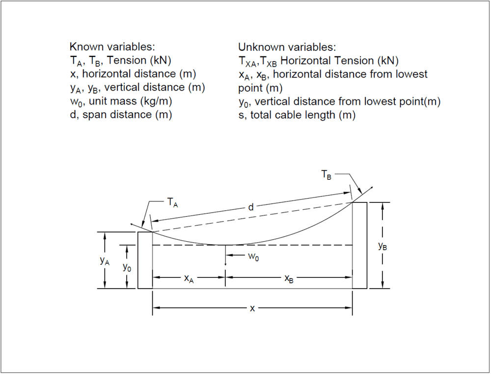
1588950855918.png

It is my understanding that the standard equation for a Catenary is: ##y = a \cdot cosh(\frac {x}{a})##. However, I feel this equation does not apply to my problem (attached pdf or figure to the right).

It seems that everywhere I look, there are Catenary problems such as this source which gives the span as well as the sag and then the problem is solved using the given variables. In my problem, I only have the span, total Tension and differential height.

The following equations are what I have tried (variables are form the source):

$$
\begin{align}
s & = c \cdot sinh(\frac {x} {c}) \\
y^2 - s^2 & = c^2 \\
W & = w_0 \cdot s \\
y & =c \cdot cosh(\frac {x} {c}) \\
T_x & =w_0 \cdot c \\
T & = w_0 \cdot y \\
\end{align}
$$

You see, my problem formulation comes from two transmission towers spaced apart at different elevations, ##P(x_a, y_a)## and ##P(x_b, y_b)##. This is throwing me off, because ultimately I figure it should be the normal equation since I have the span distance, ##d## and then simply add the formula to a line of slope ##mx+y_0##.

There are a couple of cases that I want to look into:
  1. ##T_A = T_B##, and create a solution based on this condition. Where ##y_A = y_B## as well as ## y_A \ne y_B##.
  2. Since the higher tower, ##B##, is going to have higher tension, set the known variable, ##T_B##, and solve for ##T_A## as well as a solution for sag and other parameters.
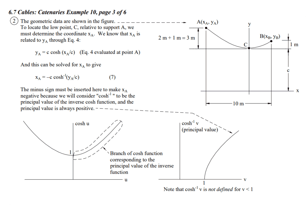
There is a similar problem in the source mentioned above, Example 10, however this problem gives a sag and solves for the tension afterwards...
1588951953296.png


The closest I feel I have come in this is the following (with my problem's variables substituted):$$ x_B = y_0 \cdot cosh^-{1}(\frac {y_B} {y_0})$$
$$ x_A = y_0 \cdot cosh^{-1}(\frac {y_A} {y_0})$$
$$ x = x_B - x_A$$
$$ y_0 \cdot cosh^{-1}(\frac {y_B} {y_0}) + y_0 \cdot cosh^{-1}(\frac {y_A} {y_0}) - x = 0$$

This equation does not take into account the Tension, someone please advise on what to do. From what I can understand, I should be able to derive and equation which I could take the limit of the T as it approached infinity, the sag should be zero.

$$\lim_{T \rightarrow +\infty} {y_0(T) = 0}$$

and another equation

$$\lim_{T \rightarrow 0} {y_0(T) = \infty}$$

Please help,

Tanner H.
 

Attachments

  • Catenary Problem.pdf
    96 KB · Views: 158
  • Like
Likes Delta2
Physics news on Phys.org
  • #2
I would start by "completing" the catenary and considering two towers of equal heights that are ##2x_B## apart. Then you know that the appropriate equation is ##y(x)=y_0\cosh\left(\dfrac{x}{y_0}\right)##. You get two equations
##y_A=y_0\cosh\left(\dfrac{x_A}{y_0}\right)##
##y_B=y_0\cosh\left(\dfrac{x_B}{y_0}\right)##
and a third equation relating the span distance to the horizontal separations by the Pythagorean theorem,
##d^2=(y_B-y_A)^2+(x_B+x_A)^2##. Are you sure the "span distance" is not the horizontal separation of the towers in which case ##d=x_B+x_A##? In either case, you have a system of three equations and three unknowns that can be solved numerically. Once you have numerical values for ##y_0##, ##x_A## and ##x_B##, you can find the tension using the "complete" catenary equation.

Disclaimer: The last time I saw the catenary equation was in grad school many, many years ago.
 
  • Like
Likes sysprog
  • #3
Thanks for your reply,

Geometrically, I agree with ## d^2 = (y_B - y_A)^2 + (x_A + x_B)^2##. I have substituted in the equations for the ##y_A## and ##y_B## and got the result below.

$$0 = y_0^2 \cdot [\cosh^2(\frac {x_B} {y_0}) -2 \cdot \cosh(\frac {x_B} {y_0}) \cosh(\frac {x_A} {y_0}) + \cosh^2(\frac {x_A} {y_0})] + (x_A + x_B)^2 - d^2$$

Ok, so I still don't understand how the tension in this problem affects the sag at all.

I am ultimately looking for an equation who's variable is only tension. I am obviously missing something. For example:

$$ y_0 = f(T) $$

Thanks,

Tanner H.
 
  • #4
Ok, I have thought about this more.. The equation I found above, assumes the center position to be ##x = x_A + x_B##. Substituting for ##x_B = x - x_A##, the result is below.

$$0 = y_0^2 \cdot [\cosh^2(\frac {x - x_A} {y_0}) -2 \cdot \cosh(\frac {x - x_A} {y_0}) \cosh(\frac {x_A} {y_0}) + \cosh^2(\frac {x_A} {y_0})] + x^2 - d^2$$

Now we still have two unknowns...

Thanks,

Tanner H.
 
  • #5
  • Like
Likes tjhollis1 and hutchphd
  • #6
I believe I have a simpler solution than the one presented in the link I gave you. Start with the catenary equation ##y(x)=a\cosh(x/a)## where ##a## is the height of the lowest point from ground zero and is not a given quantity. Given quantities are the heights of the two poles ##y_1##, ##y_2## and the horizontal pole separation ##d##. The origin of coordinates is at ground zero vertically below the lowest point on the catenary.

We write$$y=a\frac{e^{x/a}+e^{-x/a}}{2}=\frac{a}{2}\left(u+\frac{1}{u}\right)~~~~(u\equiv e^{x/a}).$$This gives the quadratic equation ##au^2-2yu+a=0## which has solutions $$u=\frac{y}{a} \pm\sqrt{\frac{y^2}{a^2}-1}.$$We identify $$e^{x/a}=u=\frac{y}{a} +\sqrt{\frac{y^2}{a^2}-1};~~~ e^{-x/a}=\frac{1}{u}=\frac{y}{a} -\sqrt{\frac{y^2}{a^2}-1}.$$It follows, by taking logaritms on both sides of the first equation, that$$x=a\ln\left(\frac{y}{a} +\sqrt{\frac{y^2}{a^2}-1}~\right).$$The separation between poles is related to ##a## by$$d=x_1+x_2=a\ln\left[\left(\frac{y_1}{a} +\sqrt{\frac{y_1^2}{a^2}-1}~\right)\left(\frac{y_2}{a} +\sqrt{\frac{y_2^2}{a^2}-1}~\right)\right].$$It pays to plot first. I chose ##y_1=11;~y_2=15;~d=16## and plotted the two sides of the equation for ##0 \leq a \leq 11##. Note that there are two solutions which can be obtained numerically (I used Mathematica). I got ##a_1=5.06## and ##a_2=8.81##. I did not investigate why there are two, it probably has something to do with the hyperbolic cosine being an even function in ##x##. Once you have ##a##, you can use ##y^2-s^2=a^2## to find the corresponding cable lengths.

I hope this helps.

Catenary.png
 
Last edited:
  • Like
Likes Delta2 and tjhollis1
  • #7
Thanks for your reply. I have thought about this over the past few days and I feel this conversation has gone off topic. I want an equation that will dictate the sag given total tension, ##T_{max}## at each end, ##d##, the space distance and, ##y_A## and ##y_B##, the height at each pole.

I see what you're doing and I was following along until I figured I should be using the equation, ## y = a * cosh(\frac {x} {a})## and follow for correctness:

For this example I am going to ignore the height difference.

$$T_x = T_{max} \cdot cosh(\phi)\\
y(x) = a \cdot cosh(\frac {x} {a})\\
\frac {d} {dx} [a \cdot cosh(\frac {x} {a})] = sinh(\frac {x} {a})\\
\phi = tan^{-1}(sinh(\frac {x} {a}))$$

Substituting...

$$T_x = T_{max} \cdot cosh(tan^{-1}(sinh(\frac {x} {a}))) \\
w \cdot a = T_{max} \cdot cosh(tan^{-1}(sinh(\frac {x} {a}))) $$

This is what I was trying to do.. The formula presents, ##a## as the function of maximum tension when solved numerically. I was just unsure how to get here. However this doesn't take into account the different height poles as the difference in height will skew the center point and thus ##x_A \ne x_B##.

I think your formula,
##d=x_1+x_2=a\ln\left[\left(\frac{y_1}{a} +\sqrt{\frac{y_1^2}{a^2}-1}~\right)\left(\frac{y_2}{a} +\sqrt{\frac{y_2^2}{a^2}-1}~\right)\right].##
will be useful in moving forward, I am just unsure of how to move forward.
 
  • #8
tjhollis1 said:
I want an equation that will dictate the sag given total tension, ##T_{max}## at each end, ##d##, the space distance and, ##y_A## and ##y_B##, the height at each pole.

I don't believe there is a single analytic expression that can give you what you want. That's because you need to solve an equation numerically. Constant ##a## is a scaling parameter that scales both ##x## and ##y##. In other words, you can express all lengths in units of ##a## instead of in meters or feet and set ##a=1## in the equations. What specifies the actual unit of length to be used is the separation between poles, ##d##. Therefore to get ##a## in the right units, you have to solve the equation relating the two as shown in post #6 and that requires a numerical solution. The tension as an input parameter does not help. You can write ##T_1=aw\cosh(x_1/a)##⁡, but you don't know the distance ##x_1## unless you first find ##a##! See below how to sort that out. Maybe you need to reformulate the model that you are trying to build.

I gave you all the pieces you need to find the tension once you have the value of ##a##, but it looks like you are uncertain about what you know and what you need to find and how. Let me walk you through a calculation and move forward from the example that I started in post #6.

You are given two vertical poles of heights ##y_1=11.0~\mathrm m## and ##y_2=15.0 ~\mathrm m## spaced distance ##d=16.0 ~\mathrm m## apart. You attach a chain between them of linear mass density ##\mu =1.50 ~\mathrm{kg/m}## and you want to calculate the tension at the poles. Fair enough?

First we solve the equation ##d=\dots## to find ##a## as I discussed in #6. We get two values, ##a_1=5.06~\mathrm m## and ##a2=8.81~\mathrm m##. We will proceed with the smaller value.

Next we find the distances ##x_1## and ##x_2## from the lowest point of the catenary.
$$x_1=a\ln\left(\frac{y_1}{a_1}+\sqrt{ \frac{y_1^2}{a_1^2}−1}\right)=5.06(\mathrm m)\ln\left(\frac{11.0}{5.06}+\sqrt{ \frac{11.0^2}{5.06^2}−1}\right)=7.14~\mathrm m \\x_2=a\ln\left(\frac{y_2}{a_1}+\sqrt{ \frac{y_2^2}{a_1^2}−1}\right)=5.06(\mathrm m)\ln\left(\frac{15.0}{5.06}+\sqrt{ \frac{15.0^2}{5.06^2}−1}\right)=8.85~\mathrm m$$Check: ##x_1+x_2=7.14~\mathrm m+8.85~\mathrm m=15.99 \mathrm m##. That's ##16.0\mathrm m## to three significant figures which is the accuracy of this calculation.

The length of the chain measured from the lowest point to any other point is given by ##s=a\sinh(x/a)##⁡. Let's find that to the tip of the poles.$$s_1=5.06(\mathrm m)\sinh(x_1/a_1)=5.06(\mathrm m)\sinh(7.14/5.06)=9.76~\mathrm m\\s_2=5.06(\mathrm m)\sinh(x_2/a_1)=5.06(\mathrm m)\sinh(8.85/5.06)=14.1~\mathrm m.$$⁡⁡⁡⁡The total length of the chain is ##s=s_1+s_2=9.76~\mathrm m+14.1~\mathrm m=23.9~\mathrm m.##

Now for the tension. Equations 5 and 6 in the source you provided are very relevant. The variable ##c## in these equations is our variable ##a##. Equation 5 says that the horizontal tension is the same no matter where you are along the catenary (that's the catenary hallmark). So,$$T_x=T_0=wa=μga_1=1.50~\mathrm{kg/m}\times 9.80~\mathrm{m/s^2}×5.06~\mathrm{m}=74.4 ~\mathrm{N}.$$Equation 6, ##T=wy##, gives the total tension in the cable. We can use it with ##y=a\cosh(x/a)##⁡ to find the total tension at each pole,$$T_1=\mu ga_1\cosh(x_1/a_1)=1.50~\mathrm{kg/m}\times 9.80~\mathrm{m/s^2}×5.06~\mathrm{m}\cosh(7.14/5.06)=162~\mathrm{N}\\T_2=\mu ga_1\cosh(x_2/a_1)=1.50~\mathrm{kg/m}\times 9.80~\mathrm{m/s^2}×5.06~\mathrm{m}\cosh(8.85/5.06)=220~\mathrm{N}.$$Knowing the total tension and the horizontal component, we can use the Pythagorean theorem to find the vertical component. Perhaps you might wish to use this as a practice template and find all of the above quantities pertinent to the other solution, ##a_2=8.81~\mathrm{m}.##
 
Last edited:
  • Like
Likes tjhollis1
  • #9
Give me some time before I dig through this, but I think you are spot on. I am using C# and utilizing Newton-Raphson solver method so I think I can reduce this down to a single equation with a single variable. Albeit, there may be two solutions but I think I can come up with an initial value equation to train the solver to guide it towards the desired solution.

I appreciate all of your help and as soon as I figure it out I will update this thread.

Thanks,

Tanner H.
 
  • #10
tjhollis1 said:
Albeit, there may be two solutions but I think I can come up with an initial value equation to train the solver to guide it towards the desired solution.
I think I am going to look into the matter of the two solutions some more myself. Perhaps we can compare notes later on.
 
  • #11
Ok, I've solved it but ohh boy is it a headache... I didn't want to, but I've solved it using multivariate Newton-Raphson method.

I decided to pick two equations that included the following variables:
  • ## T_1## or ##T_2## depending on which is higher as this is a limiting factor. As it has been proved that the higher pole holds the highest tension ##(N)##,
  • ##\Delta x##, is the horizontal separation between the poles##(m)##,
  • ##\Delta y##, is the vertical separation between the poles##(m)##,
  • ##w_o##, is the per unit mass ##(kg/m)##,
  • ##g##, gravity ##(9.81 \frac {m} {s^2})##.
The unknowns:
  • ##s##, the cable length ##(m)##,
  • ##a##, the catenary constant ##unitless##,
  • ##x_1## and ##x_2##, the horizontal length between the lowest point of the catenary ##(m)##.

These are the only variables I am to use, the rest are assumptions except for the height of each pole (##y_1## or ##y_2##), which should not affect the problem as the equation for a catenary given in the form ##y = a \cosh {\frac {x} {a}}##, if calculated at each end of the catenary, ##x_1## and ##x_2## does not yield the height ##y_1## and ##y_2## respectfully.

In reality, the first equation is derived from :

$$\begin{align} \nonumber
y(x) & = a \cosh {\frac {x} {a}} + y_0 \\
y_2 & = a \cosh {\frac {x_2} {a}} + y_0\\
y_1 & = a \cosh {\frac {-x_1} {a}} + y_0\\
\Delta x & = x_2 - x_1 \\
\Delta y & = y_2 - y_1
\end{align}$$

The first equation comes from substituting Equation ##(7)## and ##(8)## into ##(10)##, which yields the following:

$$\begin{align}
\Delta y & = a \cosh {\frac {x_2} {a}} - a \cosh {\frac {-x_1} {a}} \\
\end{align}$$

After substituting in ##\Delta x - x_2## for ##-x_1## (##x_1## was chosen here arbitrarily):
$$\begin{align}
\Delta y & = a \cosh {\frac {x_2} {a}} - a \cosh {\frac {\Delta x - x_2} {a}} \\
\end{align}$$

The next equation derives from the summation of the ##y## components of each pole's tension. We know that the summation of the weight of the catenary, ##W = w_o gs## is:

$$\begin{align}
W & = w_o g s \\
T_{1y} & = T_1 \sin {\theta_1} \\
T_{2y} & = T_2 \sin {\theta_2} \\
W & = T_{1y} + T_{2y}\\
w_o g s & = T_1 \sin {\theta_1} + T_2 \sin {\theta_2} \\
\end{align}$$

Given that the summation of horizontal forces on the catenary equal zero, another substitution can be made to reduce number of variables:

$$\begin{align}
T_{1x} & = T_1 cos(\theta_1) \\
T_{2x} & = T_2 cos(\theta_2) \\
\sum {T_x} & = 0 \\
T_1 cos(\theta_1) - T_2 cos(\theta_2) & = 0\\
T_2 cos(\theta_2) & = T_1 cos(\theta_1) \\
T_2 = T_1 \frac {cos(\theta_1)} {cos(\theta_2)} \\
\end{align}$$

Substitute ##T_1 \frac {cos(\theta_1)} {cos(\theta_2)}## for ##T_2## to get the following equation:

$$\begin{align}
w_o g s & = T_1 \sin {\theta_1} + T_1 \frac {cos(\theta_1)} {cos(\theta_2)} \sin {\theta_2} \\
w_o g s & = T_1 \sin {\theta_1} + T_1 \cos{\theta_1} \tan{\theta_2} \\
\end{align}$$

Now, there is a ways to go before this equation is complete, we still have:
  • the two angles, ##\theta_1## and ##\theta_2## and
  • the cable length, ##s##.

To eliminate the cable length, the length of the cable from the lowest point to one of the poles is generically given by ## s = a \sinh {\frac {x} {a}}##. By adding the two sides of the cable together, the following equation is yielded:

$$\begin{align}
s_2 & = a \sinh {\frac {x_2} {a}} \\
s_1 & = a \sinh {\frac {-x_1} {a}} \\
s & = s_1 + s_2 \\
s & = a \sinh {\frac {x_2} {a}} + a \sinh {\frac {-x_1} {a}}\\
s & = a \sinh {\frac {x_2} {a}} + a \sinh {\frac {\Delta x - x_2} {a}}\\
\end{align}$$

Visiting equation ##(25)## and substituting ##(30)## into ##(25)##:

$$
w_o g (a \sinh {\frac {x_2} {a}} + a \sinh {\frac {\Delta x - x_2} {a}}) = T_1 \sin {\theta_1} + T_1 \cos{\theta_1} \tan{\theta_2}
$$

Now comes the use of the derivative in post #7:

$$
\theta = \tan^{-1} \left(\sinh \left( \frac {x} {a} \right) \right)
$$

Now, this next assumption is bold, but I think is justified given that the line follows a continuous path. Since we have the vertical ##\Delta y## and horizontal ##\Delta x## distance, I assumed that the angle difference between the two is simple and addition of a constant as shown below:

$$
\Delta \theta = \tan^{-1} \left( \frac {\Delta y} {\Delta x} \right)
$$

If pole one were to be higher than pole 2, the slope of the line would be negative, therefore the resultant of the equation above will be negative and the angle of pole 1 will be higher than the angle of pole 2. The following equations can be substituted:

$$\begin{align}
\theta_1 & = \tan^{-1} \left(\sinh \left( \frac {-x_1} {a} \right) \right) - \Delta \theta\\
\theta_2 & = \tan^{-1} \left(\sinh \left( \frac {x_2} {a} \right) \right) + \Delta \theta\\
\theta_1 & = \tan^{-1} \left(\sinh \left( \frac {\Delta x - x_2} {a} \right) \right) - \tan^{-1} \left( \frac {\Delta y} {\Delta x} \right)\\
\theta_2 & = \tan^{-1} \left(\sinh \left( \frac {x_2} {a} \right) \right) + \tan^{-1} \left( \frac {\Delta y} {\Delta x} \right)\\
\end{align}$$

Okay, now we come to substitute in the above equations to get the final equation:

$$\begin{align}

T_1\left(\sin\left(\arctan\left(\sinh\left(\dfrac{x_\text{t}-x_2}{a}\right)\right)-\arctan\left(\dfrac{y_\text{t}}{x_\text{t}}\right)\right)+\tan\left(\arctan\left(\sinh\left(\dfrac{x_2}{a}\right)\right)+\arctan\left(\dfrac{y_\text{t}}{x_\text{t}}\right)\right)\cos\left(\arctan\left(\sinh\left(\dfrac{x_\text{t}-x_2}{a}\right)\right)-\arctan\left(\dfrac{y_\text{t}}{x_\text{t}}\right)\right)\right)-gm\left(\sinh\left(\dfrac{x_\text{t}-x_2}{a}\right)a+\sinh\left(\dfrac{x_2}{a}\right)a\right) = 0

\end{align}$$

So now that we have our two equations ##(12)## and ##(35)##, we may now take partials with respect to ##a## and ##x_2##.

$$\begin{align}
f_1(a, x_2) & = 0 = T_1\left(\sin\left(\arctan\left(\sinh\left(\dfrac{x_\text{t}-x_2}{a}\right)\right)-\arctan\left(\dfrac{y_\text{t}}{x_\text{t}}\right)\right)+\tan\left(\arctan\left(\sinh\left(\dfrac{x_2}{a}\right)\right)+\arctan\left(\dfrac{y_\text{t}}{x_\text{t}}\right)\right)\cos\left(\arctan\left(\sinh\left(\dfrac{x_\text{t}-x_2}{a}\right)\right)-\arctan\left(\dfrac{y_\text{t}}{x_\text{t}}\right)\right)\right)-gm\left(\sinh\left(\dfrac{x_\text{t}-x_2}{a}\right)a+\sinh\left(\dfrac{x_2}{a}\right)a\right)\\

f_2(a, x_2) & = 0 = a\cosh\left(\dfrac{x_2}{a}\right)-a\cosh\left(\dfrac{x_\text{t}-x_2}{a}\right)-y_\text{t}\\

\frac {\delta} {\delta a} \left[ f_1(a, x_2) \right] & =
T_1\left(\dfrac{\left(x_\text{t}-x_2\right)\tan\left(\arctan\left(\sinh\left(\frac{x_2}{a}\right)\right)+\arctan\left(\frac{y_\text{t}}{x_\text{t}}\right)\right)\sin\left(\arctan\left(\sinh\left(\frac{x_\text{t}-x_2}{a}\right)\right)-\arctan\left(\frac{y_\text{t}}{x_\text{t}}\right)\right)\cosh\left(\frac{x_\text{t}-x_2}{a}\right)}{\left(\sinh^2\left(\frac{x_\text{t}-x_2}{a}\right)+1\right)a^2}-\dfrac{\left(x_\text{t}-x_2\right)\cos\left(\arctan\left(\sinh\left(\frac{x_\text{t}-x_2}{a}\right)\right)-\arctan\left(\frac{y_\text{t}}{x_\text{t}}\right)\right)\cosh\left(\frac{x_\text{t}-x_2}{a}\right)}{\left(\sinh^2\left(\frac{x_\text{t}-x_2}{a}\right)+1\right)a^2}-\dfrac{x_2\sec^2\left(\arctan\left(\sinh\left(\frac{x_2}{a}\right)\right)+\arctan\left(\frac{y_\text{t}}{x_\text{t}}\right)\right)\cos\left(\arctan\left(\sinh\left(\frac{x_\text{t}-x_2}{a}\right)\right)-\arctan\left(\frac{y_\text{t}}{x_\text{t}}\right)\right)\cosh\left(\frac{x_2}{a}\right)}{\left(\sinh^2\left(\frac{x_2}{a}\right)+1\right)a^2}\right)-gm\left(-\dfrac{\left(x_\text{t}-x_2\right)\cosh\left(\frac{x_\text{t}-x_2}{a}\right)}{a}-\dfrac{x_2\cosh\left(\frac{x_2}{a}\right)}{a}+\sinh\left(\dfrac{x_\text{t}-x_2}{a}\right)+\sinh\left(\dfrac{x_2}{a}\right)\right)\\

\frac {\delta} {\delta x_2} \left[ f_1(a, x_2) \right] & = T_1\left(\dfrac{\sin\left(\arctan\left(\sinh\left(\frac{x_\text{t}-x_2}{a}\right)\right)-\arctan\left(\frac{y_\text{t}}{x_\text{t}}\right)\right)\cosh\left(\frac{x_\text{t}-x_2}{a}\right)\tan\left(\arctan\left(\sinh\left(\frac{x_2}{a}\right)\right)+\arctan\left(\frac{y_\text{t}}{x_\text{t}}\right)\right)}{a\left(\sinh^2\left(\frac{x_\text{t}-x_2}{a}\right)+1\right)}+\dfrac{\cos\left(\arctan\left(\sinh\left(\frac{x_\text{t}-x_2}{a}\right)\right)-\arctan\left(\frac{y_\text{t}}{x_\text{t}}\right)\right)\cosh\left(\frac{x_2}{a}\right)\sec^2\left(\arctan\left(\sinh\left(\frac{x_2}{a}\right)\right)+\arctan\left(\frac{y_\text{t}}{x_\text{t}}\right)\right)}{a\left(\sinh^2\left(\frac{x_2}{a}\right)+1\right)}-\dfrac{\cos\left(\arctan\left(\sinh\left(\frac{x_\text{t}-x_2}{a}\right)\right)-\arctan\left(\frac{y_\text{t}}{x_\text{t}}\right)\right)\cosh\left(\frac{x_\text{t}-x_2}{a}\right)}{a\left(\sinh^2\left(\frac{x_\text{t}-x_2}{a}\right)+1\right)}\right)-gm\left(\cosh\left(\dfrac{x_2}{a}\right)-\cosh\left(\dfrac{x_\text{t}-x_2}{a}\right)\right)\\

\frac {\delta} {\delta a} \left[ f_2(a, x_2) \right] & = \dfrac{\left(x_\text{t}-x_2\right)\sinh\left(\frac{x_\text{t}-x_2}{a}\right)}{a}-\dfrac{x_2\sinh\left(\frac{x_2}{a}\right)}{a}-\cosh\left(\dfrac{x_\text{t}-x_2}{a}\right)+\cosh\left(\dfrac{x_2}{a}\right) \\

\frac {\delta} {\delta x_2} \left[ f_2(a, x_2) \right] & =
\sinh\left(\dfrac{x_2}{a}\right)+\sinh\left(\dfrac{x_\text{t}-x_2}{a}\right)\\

\end{align}$$

What a mess and I am sure I could simplify, but, who cares when I am just going to put this into code and let it iterate.

Using the basic multivariat Newton-Raphson setup, we should be able to iterate.

\begin{displaymath} \left[\begin{array}{c}x_1 \vdots x_N\end{array}\right]_{... ... \vdots \vdots \vdots f_M({\bf x}_n) \end{array}\right] \end{displaymath}


Below is the test code I used in Python with some success (see below the code for future work):
Catenary Newton-Raphson Solver:
from numpy import *
from numpy import *
import numpy
import matplotlib.pyplot as plt

def func1(a, x_2):
    return t_1*(sin(arctan(sinh((x_t-x_2)/a))-arctan(y_t/x_t)) + cos(arctan(sinh((x_t-x_2)/a))-arctan(y_t/x_t))*tan(arctan(sinh((x_2)/a))+arctan(y_t/x_t))) - g*m*(a*sinh(x_2/a)+a*sinh((x_t-x_2)/a))

def func2(a, x_2):
    return a*cosh(x_2/a)-a*cosh((x_t-x_2)/a)-y_t

def dfunc1_da(a, x_2):
    return t_1*(((x_t-x_2)*tan(arctan(sinh(x_2/a))+arctan(y_t/x_t))*sin(arctan(sinh((x_t-x_2)/a))-arctan(y_t/x_t))*cosh((x_t-x_2)/a))/((pow(sinh((x_t-x_2)/a),2)+1)*a*a)-((x_t-x_2)*cos(arctan(sinh((x_t-x_2)/a))-arctan(y_t/x_t))*cosh((x_t-x_2)/a))/((pow(sinh((x_t-x_2)/a),2)+1)*a*a)-(x_2*pow(1/cos((arctan(sinh(x_2/a))+arctan(y_t/x_t))),2)*cos(arctan(sinh((x_t-x_2)/a))-arctan(y_t/x_t))*cosh(x_2/a))/((pow(sinh(x_2/a),2)+1)*a*a))-(g*m*((sinh((x_t-x_2)/a)+sinh(x_2/a))*a+(x_2-x_t)*cosh((x_t-x_2)/a)-x_2*cosh(x_2/a)))/a

def dfunc1_dx_2(a, x_2):
    return t_1*((sin(arctan(sinh((x_t-x_2)/a))-arctan(y_t/x_t))*cosh((x_t-x_2)/a)*tan(arctan(sinh(x_2/a))+arctan(y_t/x_t)))/(a*(pow(sinh((x_t-x_2)/a),2)+1))+(cos(arctan(sinh((x_t-x_2)/a))-arctan(y_t/x_t))*cosh(x_2/a)*pow(1/cos((arctan(sinh(x_2/a))+arctan(y_t/x_t))),2)/(a*(pow(sinh(x_2/a),2)+1))-(cos(arctan(sinh((x_t-x_2)/a))-arctan(y_t/x_t))*cosh((x_t-x_2)/a))/(a*(pow(sinh((x_t-x_2)/a),2)+1)))) - g*m*(cosh(x_2/a)-cosh((x_t-x_2)/a))

def dfunc2_da(a, x_2):
    return ((x_t-x_2)*sinh((x_t-x_2)/a))/a-(x_2*sinh(x_2/a))/a-cosh((x_t-x_2)/a)+cosh(x_2/a)

def dfunc2_dx_2(a, x_2):
    return sinh(x_2/a)+sinh((x_t-x_2)/a)##Pole 1 is higher than pole 2, thus pole one's tension is the limiting factor.
##If pole 2 is higher than pole 1, this will still solve with the tension in pole 1 as the limiting factor.
x_t = 10            ##meters
y_1 = 15            ##meters
y_2 = 13            ##meters
y_t = y_2 - y_1     ##meters
t_1 = 120           ##Newtons
g = 9.81            ##m/s^2
m = 1.00            ##kg/m

iter_max = 300
i = 0
tolerance = 1e-3
error = 1

x_2_min = 1e-6
a_min = 1e-12

x = matrix([[x_t],[x_t/2+x_2_min]])

while i < iter_max and error > tolerance:
    disp(x.T)

    J = zeros([2,2])
    f = zeros([2,1])

    J[0,0] = dfunc1_da(x[0,0], x[1,0])
    J[1,0] = dfunc2_da(x[0,0], x[1,0])

    J[0,1] = dfunc1_dx_2(x[0,0], x[1,0])
    J[1,1] = dfunc2_dx_2(x[0,0], x[1,0])

    f[0,0] = func1(x[0,0], x[1,0])
    f[1,0] = func2(x[0,0], x[1,0])

    x = x - matmul(linalg.inv(J),f)

    f[0,0] = func1(x[0,0], x[1,0])
    f[1,0] = func2(x[0,0], x[1,0])

    i = i + 1
    error = abs(numpy.max(f))
    disp("error: %.3f" % (error))

disp(x)
disp("total iterations: %i" % (i))

a = x[0,0]
x_2 = x[1,0]
x_1 = x_t - x_2
x = numpy.linspace(-x_1, x_2, 200)
y = []
y_0 = y_1 - a*cosh(-x_1/a)
for val in x:
    y.append(a*cosh((val)/a) + y_0)

plt.plot(x, y)
theta_1 = arctan(sinh((x_t - x_2)/a))-arctan(y_t/x_t)
theta_2 = arctan(sinh((x_2)/a))+arctan(y_t/x_t)
t_2 = t_1*cos(theta_1)/cos(theta_2)
plt.title("a: %.3f, x_2: %.1f, T_2: %.2f" % (a, x_2, t_2))
plt.grid(True)
plt.ylim([0, numpy.max(y)*1.05])
plt.show()
plt.close()

Figure_1.png


In this code, there are a couple of things to consider and I need your help to figure-out the following...
  • The tension must be a minimum or it will not converge. What is this value and how can one calculate the minimum tension for this to converge?
  • In the code, you will see that the variable matrix x, contains the catenary constant, ##a## in the first row (position x[0,0]) and ##x_2## in the second row (position x[1,0]).
    • The solver will not converge if the initial value of ##a## is small, however I cannot determine why. For this issue I am sure there is a way to determine the best initial guess.
    • The ##x_2##, when the tension is high enough, can be greater than ##\Delta x## which surprised me, but makes sense. I just didn't see that coming.
  • I am curious as to how we could formulate this code as such so I don't have to rewrite for the case where pole 2 is greater than pole 1. I know I could just switch the poles and the solution is the same, but my brain is fried.
I wrote this up quickly but have spent a long time on this outside of this forum. I would love your help moving forward if you could.

Thanks,

Tanner H.
 
Last edited:
  • #12
This is overwhelming to me but I will try to make some progress understanding it. I am not a Python enthusiast, FORTRAN and VBasic are my languages so I cannot comment on your code. I will make a stab at understanding how you put this together. For starters, I cannot understand why you say that ##a## is unitless. Are you saying that it's apure number like ##\pi##? If so the argument of the hyperbolic sine and cosine, ##x/a## has units of meters and that cannot be. All arguments of things like exponentials, logarithms, sines, cosines, etc. are dimensionless quantities.
tjhollis1 said:
What a mess and I am sure I could simplify, but, who cares when I am just going to put this into code and let it iterate.
It is a mess, but I think that simplifying expressions has its virtues. You must be aware of the gigo pitfall, garbage in, garbage out. How are you going to verify independently of your code that your code does what it's supposed to do?
Finally, you show a graph of a catenary. What numerical input parameters did you use to generate it? Pehraps I can use my methods to see if I can reproduce it.
 
  • #13
Wait, hold on...

It works only if trained initial guesses. That is the main problem. It looks like there are tons of solutions to each given. I am traveling tomorrow and I am putting this down for now. Please don't look further into this until I can sort out why the behavior of the convergence is so dependent upon the initial guess.

To answer your question about the constant, ##a##, I was mislead by the fact it is a constant. Usually constants are unitless, thanks for catching that.

To answer the graph comment, I updated the code after the fact and forgot to update the graph that included the solver's final conditions.

I am testing against verified problems, here.

Thanks,
Tanner H.
 
  • #14
Safe travels. Meanwhile I wll compile a list of observations and comments to post #11 that could be discussed upon your return.
 
  • #16
Comments and observations on post #11

1. In equation (7) you write ##y(x) = a \cosh {\frac {x} {a}} + y_0##. What is ##y_0## and why is it necessary to have it? When ##x=0## the equation predicts that ##y(0)=a+y_0##. I assume that this is a typo.

2. Equations 13-17 are correct. However, the trig functions involving angle ##\theta## can be simplified. The slope of the curve at some value of ##x## is $$\tan\theta=\frac{dy}{dx}=\frac{d}{dx}\left[a \cosh\left(\frac{x}{a}\right)\right]=\sinh\left(\frac{x}{a}\right)=\frac{s}{a}.$$This suggests a right triangle as shown below. Note that the hypotenuse is ##y## and that the Pythagorean theorem is satisfied in accordance with equation 2 in post #1 (with ##c=a##).
CatenaryTriangle.png

From the triangle we deduce that ##\sin\theta=\dfrac{s}{y};~~\cos\theta=\dfrac{a}{y}.##

3. You have missed an important equation which is obtained by demanding that a segment of the catenary from the lowest point (##y=a##) to an arbitrary point ##y## must be in equilibrium. From the free body diagram shown below
CatenaryFBD.png

Horizontal equilibrium: ##T \cos\theta=T_0##
Vertical equilibrium: ##T\sin\theta=w_0s##
Divide the bottom equation by the top to get ##\tan\theta=\dfrac{w_0s}{T_0}=\dfrac{s}{a}~\rightarrow~T_0=w_0a##.
The total tension is $$T=\frac{T_0}{\cos\theta}=\frac{w_0a}{\frac{a}{y}}=w_0y=w_0a\cosh(x/a)$$The components of the tension are$$T_x=T\cos\theta=w_0y\times \frac{a}{y}=w_0a=\text{constant}\\T_y=T\sin\theta=w_0y\times\frac{s}{y}=w_0s=w_0 a\sinh(x/a)$$Note that the right triangle formed by ##T##, ##T_x## and ##T_y## is similar to the right triangle shown above. Their sides are proportional to each other with the constant of proportionality being ##w_0##,$$T=w_0y;~T_x=w_0 a;~ T_y=w_0 s.$$4. The most important realization you should come to is that angle ##\theta## is irrelevant so stop trying to find expressions for it. What you care about are the trig functions of ##\theta## and these you have either in terms of ratios of sides in the length triangle or in the tension triangle. That will simplify your code and preserve your sanity. My advice is to toss out everything past equation (17) and start over again.

5. Is your goal to find a single equation relating given parameters ##T_A##, ##T_B##, ##y_A##, ##y_B##, ##x_A+x_B##, ##w_0## with unknown parameter ##a## and solve that equation to find ##a##? If so, please note that the tensions ##T_A## and ##T_B## are redundant as given parameters because ##T_A=w_0y_A## and ##T_B=w_0y_B##. So really this goal is to find a single equation relating given parameters ##y_A##, ##y_B##, ##x_A+x_B##, ##w_0## to unknown parameter ##a##. But this goal was reached in post #6. Furthermore, in post #8 I showed you how to solve for ##a## and determine the rest of the unknown quantities. If you agree that this is your goal, then your task is to write code to solve the equation in post #6 and calculate the rest of the unknown quantities.

If this is not your goal, then please specify what your goal is so that I can see if there is something I can do to help you reach it. I hope I have convinced that the tensions are useless as input parameters if you know the pole heights and the linear weight density.
 
Last edited:
  • #17
kuruman said:
How are you going to verify independently of your code that your code does what it's supposed to do?
Since the OP is already writing iterative optimization code, one way to verify it is a simple mass-spring-simulation, which will definitely converge towards a unique solution here.
 
Last edited:
  • #18
A.T. said:
Since the OP is already writing iterative optimization code, one way to verify it is a simple mass-spring-simulation, which will definitely converge towards a unique solution here.
Sure, but that will test only the "iterative optimization" part of the code under the assumption that what goes in is correct. I am not yet convinced that OP has a clear picture of what it is that should go in and that it is properly formulated in this other case that is a completely different problem from a mass-spring system.
 

1. What is the "Unsolvable Catenary Problem"?

The "Unsolvable Catenary Problem" is a mathematical problem that involves finding the shape of a hanging chain or cable suspended between two points under the influence of gravity. It is called "unsolvable" because there is no algebraic or closed-form solution to this problem.

2. Why is the "Unsolvable Catenary Problem" important?

The "Unsolvable Catenary Problem" is important because it has practical applications in engineering and physics. The shape of a hanging chain or cable can affect the stability and strength of structures such as bridges and suspension cables. Understanding and solving this problem can lead to more efficient and safe designs.

3. Who first studied the "Unsolvable Catenary Problem"?

The "Unsolvable Catenary Problem" was first studied by mathematicians such as Galileo, Huygens, and Leibniz in the 17th century. However, the problem was not fully understood until the 18th century when mathematicians like Johann Bernoulli and Leonhard Euler made significant contributions to its solution.

4. Can the "Unsolvable Catenary Problem" be solved numerically?

Yes, the "Unsolvable Catenary Problem" can be solved numerically using methods such as the finite element method or the method of relaxation. These methods involve dividing the catenary into small segments and using iterative calculations to approximate its shape.

5. Are there any real-life examples of the "Unsolvable Catenary Problem"?

Yes, there are many real-life examples of the "Unsolvable Catenary Problem" such as the shape of a hanging cable or wire, the shape of a suspension bridge, and the shape of a hanging rope or chain. It also applies to other natural phenomena such as the shape of a spider web or the shape of a hanging plant.

Similar threads

  • Classical Physics
Replies
3
Views
676
  • Classical Physics
Replies
3
Views
1K
Replies
5
Views
367
  • Calculus and Beyond Homework Help
Replies
2
Views
453
Replies
4
Views
1K
Replies
2
Views
4K
  • Calculus and Beyond Homework Help
Replies
3
Views
1K
  • Introductory Physics Homework Help
Replies
6
Views
221
  • Classical Physics
Replies
0
Views
110
  • Classical Physics
Replies
1
Views
2K
Back
Top