A Constructing PDFs for Max Likelihood Density Estimation Problem

[AEW]

TL;DR

Construct some probability density functions for the maximum likelihood density estimation problem.

I have the following constrained optimization problem corresponding to the maximum likelihood density estimation:
$$
\begin{aligned}
&\text{maximize} && L(f) \\
&\text{subject to} && f \in H \\
&&& \int_a^b f(x) \mathop{}\!\mathrm{d} x = 1 \\
&&& f(x) \geq 0 \text{ for all } x \in [a,b].
\end{aligned}
$$
where $x$ is a random variable with probability density function (PDF) $f$ on an interval $[a,b] \subset \textrm{IR}$, and $H$ is a subspace of $L^1 [a,b]$ (i.e., Lebesgue integrable on $[a,b]$).

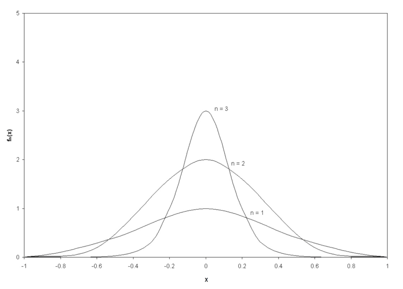
I need to construct some PDFs $f_n$ to prove the existence of a solution to the above optimization problem, which should have the following properties:
- Continuous and positive on the interval $(-1,1)$,
- Integrates to one on the interval $[-1,1]$,
- Vanishes at $(-1)$ and $1$,
- Equal to $n$ at $x=0$ (e.g., $f_2=2$ at $x=0$).

These functions $f_n$ are graphically represented in the figure below. My question is how to mathematically represent the functions $f_n$.

Thanks.

 

[andrewkirk]

The PDFs of the beta distribution have all but one of the properties you want, on the interval [0,1], provided you choose $\alpha = \beta$. That leaves one free parameter you can use to set the summit of each curve at the level you want.
If you select a family of betas with peak heights at the even integers, you can then just transpose them to the interval [-1,1] and halve their height to get what you need.

 

[AEW]

The PDFs of the beta distribution have all but one of the properties you want, on the interval [0,1], provided you choose $\alpha = \beta$. That leaves one free parameter you can use to set the summit of each curve at the level you want.
If you select a family of betas with peak heights at the even integers, you can then just transpose them to the interval [-1,1] and halve their height to get what you need.

Thank you, @andrewkirk, for your answer. That was helpful.