lefty
- 5
- 7
- TL;DR
- The paper, "Numerical Analysis of Coleman-de Luccia Tunneling" describes a fascinating scenario for instantiating a bubble universe from a primal quantum field that I would like to understand but I'm not able to successfully solve the boundary value problem.
I am studying the paper Numerical Analysis of Coleman-de Luccia Tunneling in which the authors describe a quantum tunneling event from a false vacuum to a true vacuum of a quantum field ##\phi(\tau)## with potential ##V(\phi)## having a spacetime geometry defined by ##a(\tau)##. This tunneling event is proposed as a possible mechanism for instantiating a bubble universe. As per section 4.1, let the field potential be:
##\displaystyle V(\phi)=v_0+\frac{v_1}{\cosh(\phi/m)}+v_2\tanh(\frac{\phi}{m})##
Then the underlying quantum field equation is:
##\displaystyle \ddot{\phi}+3\frac{\dot{a}}{a}\dot{\phi}=\frac{dV}{d\phi}##
And the spacetime geometry ##a(\tau)## of the instanton given by :
##\displaystyle \ddot{a}=-\frac{a}{3 M^2}\left(\dot{\phi}^2+V\right)##
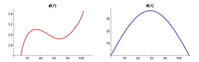
And according to the paper, these equation are solved as BVPs with ##a(0)=0##, ##\dot{a}(0)=1##, ##\dot{\phi}(0)=0## and the object of the exercise is to find a starting value for ##\phi(0)=\phi_0## in which ##a(\tau_{max})=0## then check if ##\dot{\phi}(\tau_{max})=0##. If not, then adjust ##\phi_0## and repeat. Successfully solving the equations leads to an instanton that looks like Figure 3 in the paper. Letting ##v_0=v_1=v_2=1##, ##m=1## and ##M=30##, I'm able to arrive at the right geometry. The plot below is one example of the solution I obtain. Other solutions I obtain by varying the parameters result in Fourier-type oscillations of ##\phi(\tau)##. The instanton through the field should be a smooth tunneling from the false vacuum to the true vacuum as per Figure 3. The blue plot of the spacetime geometry is generally correct but the field perturbation of the instanton shown in red is not correct as per Figure 3 in the paper.
I can post my Mathematica code if this is something others here would be interested in helping me with. I'm mostly interested in solving the differential equations and successfully obtaining the instanton given by ##\{\phi(\tau),a(\tau)\}## shown in Figure 3.
##\displaystyle V(\phi)=v_0+\frac{v_1}{\cosh(\phi/m)}+v_2\tanh(\frac{\phi}{m})##
Then the underlying quantum field equation is:
##\displaystyle \ddot{\phi}+3\frac{\dot{a}}{a}\dot{\phi}=\frac{dV}{d\phi}##
And the spacetime geometry ##a(\tau)## of the instanton given by :
##\displaystyle \ddot{a}=-\frac{a}{3 M^2}\left(\dot{\phi}^2+V\right)##
And according to the paper, these equation are solved as BVPs with ##a(0)=0##, ##\dot{a}(0)=1##, ##\dot{\phi}(0)=0## and the object of the exercise is to find a starting value for ##\phi(0)=\phi_0## in which ##a(\tau_{max})=0## then check if ##\dot{\phi}(\tau_{max})=0##. If not, then adjust ##\phi_0## and repeat. Successfully solving the equations leads to an instanton that looks like Figure 3 in the paper. Letting ##v_0=v_1=v_2=1##, ##m=1## and ##M=30##, I'm able to arrive at the right geometry. The plot below is one example of the solution I obtain. Other solutions I obtain by varying the parameters result in Fourier-type oscillations of ##\phi(\tau)##. The instanton through the field should be a smooth tunneling from the false vacuum to the true vacuum as per Figure 3. The blue plot of the spacetime geometry is generally correct but the field perturbation of the instanton shown in red is not correct as per Figure 3 in the paper.
I can post my Mathematica code if this is something others here would be interested in helping me with. I'm mostly interested in solving the differential equations and successfully obtaining the instanton given by ##\{\phi(\tau),a(\tau)\}## shown in Figure 3.
