How can I linearize my (negative slope) quadratic graph?

In summary, the conversation revolves around an investigation of the relationship between distance and sag of a beam. The determined relationship is not linear but can be linearized using the natural logarithm. The data points collected from trials are used to create a polynomial equation to represent the relationship. However, when the data is graphed on a logarithmic scale, there are discrepancies and errors. The speaker is seeking help to understand what went wrong and to complete their report.
  • #1
utp9
12
2
TL;DR Summary
Solve an equation of power through a linear graph.
I am doing an investigation of how much a beam sags, based on the distance from its midpoint.
This is my hypothetical equation:

The relationship between distance, d and sag, s is not a linear relationship. Below, is the determined relationship between the variables, linearized by natural logarithm.[1]
\begin{align*}
s &∝ d^t & \quad &s = \text{vertical sag(mm)}\\
s &= ud^t &\text{(equation one)}\quad &d = \text{distance(mm)}\\
\ln(s) &= \ln(ud^t) & \quad &u = \text{constant}\\
\ln(s) &= t\ln(d) + \ln(u) &\text{(equation two)} \quad & t = \text{constant}\\
\end{align*}
These are my data points:
Sag of the beam
s / mm
∆mm = ±1.0​
Distance
d / mm
∆mm = ±0.5​
Trial 1​
Trial 2​
Trial 3​
Trial 4​
Mean sag
s / mm​
0.0​
35.0​
36.0​
36.0​
35.0​
35.5 ±0.5​
50.0​
34.0​
36.0​
35.0​
34.5​
34.9 ±1.0​
100.0​
32.5​
33.0​
33.5​
33.5​
33.1 ±0.5​
150.0​
29.0​
30.0​
30.0​
29.0​
29.5 ±1.0​
200.0​
26.0​
27.0​
26.5​
27.0​
26.6 ±0.5​
250.0​
22.0​
23.0​
22.0​
22.5​
22.4 ±0.5​
300.0​
17.0​
17.0​
17.0​
17.0​
17.0 ±0.0​

I get this polynomial(to the second degree) of these points:
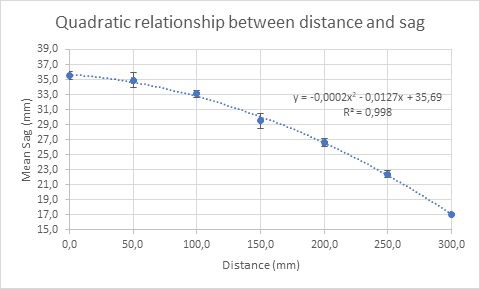
1582458232910.png


Applying ln-ln to the x and y-axis gets me these data points:
Distance
d / mm
∆mm = ±0.5​
Ln(d)​
Mean sag
s / mm​
Ln(s)​
0.0​
UND*​
35.5 ±0.5​
3.6 ±0.0​
50.0​
3,9​
34.9 ±1.0​
3.6 ±0.0​
100.0​
4,6​
33.1 ±0.5​
3.5 ±0.0​
150.0​
5,0​
29.5 ±1.0​
3.4 ±0.0​
200.0​
5,3​
26.6 ±0.5​
3.3 ±0.0​
250.0​
5,5​
22.4 ±0.5​
3.1 ±0.0​
300.0​
5,7​
17.0 ±0.0​
2.8 ±0.0​
*As ln(0) is not a real number, the distance 0.0mm will not be included in the graph

My "linear" graph looks like this:
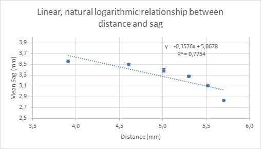
1582458341170.png

With the graph, ln(u) is my y-intercept and t is my gradient to complete the equation in my hypothesis.

My question:
I cannot figure out what is going wrong as everything should work in this situation. I have 10 pages of report ready except for this last graph and conclusion based off the graph.
I've spent hours yesterday attempting to understand what is going wrong, if anyone can help or needs more information please comment.

[1] “Getting Straight Line Graphs.” Physics for the IB Diploma Exam Preparation Guide, by K. A. Tsokos, Cambridge University Press, 2016, p. 5.
 
Last edited:
Physics news on Phys.org
  • #2
It looks like you have your results on a spreadsheet, which take the effort out of trying different graphs. So try plotting s against d2. Each side of your equation 1 is equal (i.e. it's an equation) so s and d2 should be proportional everywhere. The slope of the graph will be what?? (Exercise for the student).
Equation 2 should be a straight line if the relationship is a simple power (gradient t) law and the intercept will be offset by ln(u) - which is a constant.
Sorry if I'm 'talking down' to you as the general principle of re-drawing results graphs to get a recognisable straight line, is well known. The scatter will show random errors and/or deviations from a simple law.
 
  • #3
The way you describe the problem suggests that the errors could be talking. The line on the graph is not far from the 50mm reading so you are asking how can the sag be far off the line? Perhaps you could work it backwards and find what distance produces a sag of 34.9. Sometimes changing to a log scale can produce unexpected 'stretching'. The original graph has a very small slope at 50mm, which would / could produce that stretching effect although the log log graph hides it. Look at the error bars you drew and explore what happens over the range of those bars, working backwards.
 
  • #4
sophiecentaur said:
The way you describe the problem suggests that the errors could be talking. The line on the graph is not far from the 50mm reading so you are asking how can the sag be far off the line? Perhaps you could work it backwards and find what distance produces a sag of 34.9. Sometimes changing to a log scale can produce unexpected 'stretching'. The original graph has a very small slope at 50mm, which would / could produce that stretching effect although the log log graph hides it. Look at the error bars you drew and explore what happens over the range of those bars, working backwards.

I had accidentally used a different graph in my previous reply (which I didn't delete fast enough). I plotted it using the same dataset as my original graph, but reversed the y values.

Now onto what we discussed: From what I understood, I plotted two graphs:
ln(d)^2 and ln(d^2). However, they both looked almost the same as my original graph:
1582465533731.png

1582465540637.png

What doing wrong?Deleted reply:

Thanks a lot for the response, this is my first time really working with graphs.

I got this line which looks better:
Imposter linear graph.png

However, when I plug it into my equation:
ln(s) = tln(d) + ln(u)

ln(u) = 1,0788 (y-intercept)

t=0,4409

ln(s) = 0,4409 ln(d) + 1,0788

s = udt

u = e^1,0788= 2.9411

s = 2.9411d^0,4409I try and insert a distance i.e. 50mm: s = 2.9411*50^0,4409

I get an answer of s = ~16.5mm, which is completely off my measured 34.9mm.
Could you provide some insight on what's happening here?
 
Last edited:
  • #5
How are you defining sag? According to your original equation sag=0 at d=0. Not sure what you are doing here, so please elucidate.
 
  • #6
hutchphd said:
How are you defining sag? According to your original equation sag=0 at d=0. Not sure what you are doing here, so please elucidate.

utp9 said:
s=ud^t
That is my equation for sag. My power of t didn't transfer over from word, sorry.

For my investigation sag is the amount of vertical depression the beam endures when applying a mass at different points from the midpoint of the beam. Distances of: 0.0, 50.0 100.0, 150.0, 200.0, 250.0, and 300.0 (mm)

Do you need any more information?
 
Last edited:
  • #7
I'm confused as to the geometry. How long is the beam? Is it supported at the ends or cantilevered? Your data looks good but not for the experiment I have in my head...
 
  • #8
hutchphd said:
I'm confused as to the geometry. How long is the beam? Is it supported at the ends or cantilevered? Your data looks good but not for the experiment I have in my head...

The beam is a double overhanging beam of 1000mm with 50mm overhanging each end. So, 900mm between the two pivot points.

My diagram:
1582480320629.png
 
  • #10
I have spent some time with my problem.
Here is a summary of where I'm currently at.

When reversing my graph's y-axis I can almost get an almost perfect line. This line gives me the correct slope and intercept, if I insert the distance in reverse.
i.e. if I insert 50mm distance into my equation I will get the result for 300mm, 100m gives 250mm result, etc.

ln(s) = tln(d) + ln(u)
ln(u) = 1,1824 (y-intercept)
t=0,4204
ln(s) = 0,4204*ln(d) + 1,1824
s = udt
u = e^1,18248= 3.2621
s = 2.9411d3.2621

i.e. d = 50mm
2.9411*503.2621 = 16.9mm which corresponds to sag for 300mm
2.9411*2503.2621 = 33.2mm which corresponds to sag for 100mm

Here is said graph:
1582484799611.png

ln(Distance (mm))ln(Mean Sag (mm))
5,7
3,6​
5,5
3,5​
5,3
3,4​
5,0
3,3​
4,6
3,1​
3,9
2,8​
(In original graph 3,9 was first and 5,7 was last, others were reversed as well

Now, how can I get a correct result?
 

Attachments

  • 1582484425661.png
    1582484425661.png
    4.4 KB · Views: 326
Last edited:
  • #11
What is a general statement of the problem?

As I understand it, you can fit an equation of the form ##s = Ad^2 + Bd + C ## to the data for sag ##s## vs distance ##d##. Given this fact, do you expect that plotting ##x = ln(s)## as a function of ##y = ln(d^2)= 2 ln(d)## will be a straight line?

If ##s = Ad^2## (with no terms ##Bd## and ##C## ) then, yes, ##ln(s) = ln(Ad^2) = ln(A) +2 ln(d)## is a linear equation in the variables ##ln(s)## and ##ln(d)##. However, if ##B## and ##C## are not zero then we are working with ##ln(s) = ln(Ad^2 + Bd + C)## which does not simplify to a linear equation.

If you want to get a linear equation by taking the logs of both sides of another equation, you can try transforming the variables in some way before taking their logs. Does the reference you cited treat this topic? What does it say about getting straight line graphs?
 
  • Like
Likes hutchphd
  • #12
Stephen Tashi said:
What is a general statement of the problem?

My problem: In my hypothesis I state that the equation to solve is s = u*dt and I need to solve u and t.

Stephen Tashi said:
As I understand it, you can fit an equation of the form s=Ad2+Bd+Cs=Ad2+Bd+Cs = Ad^2 + Bd + C to the data for sag sss vs distance ddd. Given this fact, do you expect that plotting x=ln(s)x=ln(s)x = ln(s) as a function of y=ln(d2)=2ln(d)y=ln(d2)=2ln(d)y = ln(d^2)= 2 ln(d) will be a straight line?

Honestly, i didn't quite understand how that would help, I just tried something I was suggested.

Stephen Tashi said:
Does the reference you cited treat this topic? What does it say about getting straight line graphs?

I'm basing this part of my research on my physics textbook which says this:
IMG_1633.JPG

Also, off of this previous IA: https://docs.wixstatic.com/ugd/e2ae59_ace5b2c6978a4cea99c24faf32eae837.pdf

If possible could you provide some insight to my previous reply on this thread?
This is the first time I'm attempting graphical analysis so I am learning the topic as I go.
 
  • #13
Thanks for the drawing.

Just looking at your data it is clear that the displacement should be measured relative to the maximum value (35.0mm), so your quadratic hypothesis should use this relative displacement. Your original quadratic supposition should define "s" as relative displacement. As I mentioned previously your original proportionality s∝dt requires d=0 to give s=0 so clearly you need to start there. Otherwise this is hopeless from the start!
 
  • #14
utp9 said:
ln(s) = tln(d) + ln(u)
ln(u) = 1,1824 (y-intercept)
t=0,4204
ln(s) = 0,4204*ln(d) + 1,1824
s = udt
##s = u d^t##
u = e^1,18248= 3.2621
s = 2.9411d3.2621
##s = 3.2631 d^{0.4204}##
 
  • #15
If you try to put log(0) on your graph, you will need a very big piece of paper. Not a problem if you measure from another ‘undeflected’ origin. But log graphs are not necessarily best for all situations because of the compression of the high numbers in the range. Have you ever seen log / log graph paper? It may not be around these days. Try googling and you’ll see how 1 to 10 is the same width as 10 to 100 and 100 to 1000. Great for some applications but need to be used with caution.
 
  • Like
Likes hutchphd
  • #16
utp9 said:
If possible could you provide some insight to my previous reply on this thread?

Your replies are difficult to understand. Try beginning the description of a problem with a "topic sentence" that states an overview of the problem.

When your data is plotted as ##(\ln(s), \ln(d))## can you closely fit a straight line to it or not? From your previous posts, I can't tell. In post #4, is the material after "deleted reply:" supposed to be something you want deleted?

The goal of your graphical analysis is find a transformation of the data that makes a straight line. If the ##(s,d)## data is not consistent with the hypothesis ##s = ud^t## then no sort of transformation of the data will support the hypothesis that ##s = ud^t##. If you find a way of transforming the data that gives a nice straight line, you should change the hypothesis to something that is consistent with that transformation.

As to your previous post, it isn't clear what you are doing. You speak of reversing the Y-axis and you also say "if I reverse the distance", which is something plotted on the x-axis. State the format of the data you are plotting. What does "reversing" mean mathematically? Is the format ##(\ln(s), ln(2m -d))## where ##m## is the midvalue of the distance measurements? Or perhaps it's ##(\ln(s), 2m - \ln(d))## where ##m## is the midvalue of the natural log of distance measurements?

If you aren't plotting ##ln(d)## on the x-axis then change the label for the x-axis to indicate what is being plotted.

Let's suppose that we can fit a straight line to the format ##(\ln(s),ln(2m-d))##.
So we have ##ln(s) = A \ln(2m -d) + B ##. The hypothesis this supports is ## e^{\ln(s)} = e^{A \ln(2m-d) + B}## which is equivalent to ##s = u(2m-d)^t ## where ##u = e^B##, ##m##, and ##t = A## are constants. I don't think this describes what you actually did. It only illustrates the idea that you must change your hypothesis to match whatever was done in transforming the data.
 
  • #17
hutchphd said:
Thanks for the drawing.

Just looking at your data it is clear that the displacement should be measured relative to the maximum value (35.0mm), so your quadratic hypothesis should use this relative displacement. Your original quadratic supposition should define "s" as relative displacement. As I mentioned previously your original proportionality s∝dt requires d=0 to give s=0 so clearly you need to start there. Otherwise this is hopeless from the start!
Stephen Tashi said:
Your replies are difficult to understand. Try beginning the description of a problem with a "topic sentence" that states an overview of the problem.

When your data is plotted as ##(\ln(s), \ln(d))## can you closely fit a straight line to it or not? From your previous posts, I can't tell. In post #4, is the material after "deleted reply:" supposed to be something you want deleted?

The goal of your graphical analysis is find a transformation of the data that makes a straight line. If the ##(s,d)## data is not consistent with the hypothesis ##s = ud^t## then no sort of transformation of the data will support the hypothesis that ##s = ud^t##. If you find a way of transforming the data that gives a nice straight line, you should change the hypothesis to something that is consistent with that transformation.

As to your previous post, it isn't clear what you are doing. You speak of reversing the Y-axis and you also say "if I reverse the distance", which is something plotted on the x-axis. State the format of the data you are plotting. What does "reversing" mean mathematically? Is the format ##(\ln(s), ln(2m -d))## where ##m## is the midvalue of the distance measurements? Or perhaps it's ##(\ln(s), 2m - \ln(d))## where ##m## is the midvalue of the natural log of distance measurements?

If you aren't plotting ##ln(d)## on the x-axis then change the label for the x-axis to indicate what is being plotted.

Let's suppose that we can fit a straight line to the format ##(\ln(s),ln(2m-d))##.
So we have ##ln(s) = A \ln(2m -d) + B ##. The hypothesis this supports is ## e^{\ln(s)} = e^{A \ln(2m-d) + B}## which is equivalent to ##s = u(2m-d)^t ## where ##u = e^B##, ##m##, and ##t = A## are constants. I don't think this describes what you actually did. It only illustrates the idea that you must change your hypothesis to match whatever was done in transforming the data.
sophiecentaur said:
If you try to put log(0) on your graph, you will need a very big piece of paper. Not a problem if you measure from another ‘undeflected’ origin. But log graphs are not necessarily best for all situations because of the compression of the high numbers in the range. Have you ever seen log / log graph paper? It may not be around these days. Try googling and you’ll see how 1 to 10 is the same width as 10 to 100 and 100 to 1000. Great for some applications but need to be used with caution.
Just for some closure, I consulted my teacher and was able to explain thing a bit better in person. You were all correct and there was no way to linearize the graph. My hypothesis was wrong.

Through the graphical analysis, the actual relationship was quadratic and there was no power relationship,
 
  • Like
Likes Stephen Tashi and hutchphd

1. How do I determine the equation of a quadratic graph with a negative slope?

To determine the equation of a quadratic graph with a negative slope, you will need to use the general form of a quadratic equation, y = ax^2 + bx + c, where a, b, and c are constants. The coefficient 'a' will be negative in this case, indicating a negative slope. You can then use the coordinates of any two points on the graph to solve for the remaining constants and obtain the equation.

2. Can I use the same method to linearize a negative slope quadratic graph as I would for a positive slope quadratic graph?

Yes, the same method can be used to linearize a negative slope quadratic graph as you would for a positive slope quadratic graph. You will need to find the inverse of the quadratic equation, which will give you a linear equation in the form of y = mx + b. The slope, m, will be negative in this case, indicating a negative slope.

3. What is the purpose of linearizing a negative slope quadratic graph?

The purpose of linearizing a negative slope quadratic graph is to transform it into a linear equation, which is easier to work with and interpret. This makes it easier to analyze the data and make predictions based on the trend of the graph.

4. Can I use a different method to linearize a negative slope quadratic graph?

Yes, there are multiple methods that can be used to linearize a negative slope quadratic graph, such as using logarithmic or exponential functions. However, the most commonly used method is finding the inverse of the quadratic equation as it results in a linear equation.

5. Is it possible to have a negative slope on a quadratic graph?

Yes, it is possible to have a negative slope on a quadratic graph. This indicates that the graph is decreasing as the x-values increase. In contrast, a positive slope on a quadratic graph would indicate that the graph is increasing as the x-values increase.

Similar threads

  • MATLAB, Maple, Mathematica, LaTeX
Replies
5
Views
7K
Back
Top