Solving 2nd order differential equation numerically

[tejsa1]

I'm writing a paper about the projectile motion with the consideration og air resistance - I have obtained two formulas:
a_x = k*(v_x²+v_y²)^0.5 * v_x
a_y = k*(v_x²+v_y²)^0.5 * v_y - g

(K and g are constants; K = -0,02, g =9,82)
I cand write these two as 2 different differential equations:
v'x(t) = k*(v_x(t)²+v_y(t)²)^0.5 * v_x(t)
x''(t) = k*(_x(t)²+v_y(t)²)^0.5 * v_x(t)

v'y(t) = k*(_x(t)²+v_y(t)²)^0.5 * v_y(t) - g
y''(t) = k*(_x(t)²+v_y(t)²)^0.5 * v_y(t) - g

start values:
v_x(0) = 5.736
v_y(0) = 8.192
x(0)=0
y(0)=0

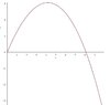
I would like to make solve the equations numerically and get a (t,x(t))-graph and (t,y(t))-graph

My problem is I really can't see how I'm going to use Runga-kutta method on the equations - Can anyone help?

 

[Ackbach]

So, RK4 is meant to apply to the ODE $\dot{r}=f(t,r), \; r(t_0)=r_0$, where $r$ could be vector or scalar. In your case, it's a vector, call it $\mathbf{r}$. Moreover, since your original DE is second-order, we're really going to have four components to the vector. Let's define things carefully. We define:
\begin{align*}
r_1&:=x \\
r_2&:=y \\
r_3&:=v_x \\
r_4&:=v_y.
\end{align*}
Then what is the ODE governing $r$? Well, we have the following:
$$\dot{\mathbf{r}}=\begin{bmatrix}\dot{r}_1 \\ \dot{r}_2 \\ \dot{r}_3 \\ \dot{r}_4\end{bmatrix}
=\begin{bmatrix}r_3 \\ r_4 \\ k r_3\sqrt{r_3^2+r_4^2} \\ k r_4\sqrt{r_3^2+r_4^2} - g \end{bmatrix}
=f(t,\mathbf{r}).$$
So far, all I've done is define some new variables, and substitute into be consistent with your original ODE. I've also reduced the ODE to first-order using the usual method. The initial condition is going to be
$$\mathbf{r}_0=\mathbf{r}(t_0)=\begin{bmatrix} 0 \\ 0 \\ 5.736 \\ 8.192\end{bmatrix}.$$

Now, The Runga-Kutta Method (RK4), works like this:

Choose a step size $h$. Define
\begin{align*}
\mathbf{r}_{n+1}&=\mathbf{r}_n+\frac{h}{6}(k_1+2k_2+2k_3+k_4) \\
t_{n+1}&=t_n+h, \qquad \text{where} \\
k_1&=f(t_n,\mathbf{r}_n) \\
k_2&=f\left(t_n+\frac{h}{2},\mathbf{r}_n+\frac{h}{2} \, k_1\right) \\
k_3&=f\left(t_n+\frac{h}{2},\mathbf{r}_n+\frac{h}{2} \, k_2\right) \\
k_4&=f\left(t_n+h,\mathbf{r}_n+h k_3\right).
\end{align*}

So you can see that this is a sort of cascading, bootstrapping sort of method. You find the initial conditions, compute $k_1$, then you can compute $k_2$, then $k_3$, then $k_4$, then $\mathbf{r}_{n+1}$. You'll note that the $k_j$ are all vectors, the result of plugging things into $f$ defined above. All the operations are defined, since you just have scalar multiplication and vector addition.

Does this help?

 

[tejsa1]

Thanks for the extremely adequate answer!
But I still haven't figured it out. I don't understand how to calculate k1, k2, k3 and k4 - can you give me one example please? :D

 

[Ackbach]

All right, here goes. Let's pick a step size of $h=0.1$. The ODE is actually autonomous (no $t$ shows up explicitly in the ODE), so we can simplify the notation slightly to obtain
$$\dot{\mathbf{r}}=\begin{bmatrix}\dot{r}_1 \\ \dot{r}_2 \\ \dot{r}_3 \\ \dot{r}_4\end{bmatrix}
=\begin{bmatrix}r_3 \\ r_4 \\ k r_3\sqrt{r_3^2+r_4^2} \\ k r_4\sqrt{r_3^2+r_4^2} - g \end{bmatrix}
=f(\mathbf{r}),$$
and
\begin{align*}
\mathbf{r}_{n+1}&=\mathbf{r}_n+\frac{h}{6}(k_1+2k_2+2k_3+k_4) \\
t_{n+1}&=t_n+h, \qquad \text{where} \\
k_1&=f(\mathbf{r}_n) \\
k_2&=f\left(\mathbf{r}_n+\frac{h}{2} \, k_1\right) \\
k_3&=f\left(\mathbf{r}_n+\frac{h}{2} \, k_2\right) \\
k_4&=f\left(\mathbf{r}_n+h k_3\right).
\end{align*}
The initial condition, again, is
$$\mathbf{r}_0=\mathbf{r}(t_0)=\begin{bmatrix} 0 \\ 0 \\ 5.736 \\ 8.192\end{bmatrix}.$$
So, the first order of business is to compute $k_1$:
$$k_1=f(\mathbf{r}_0)=\begin{bmatrix}5.736 \\ 8.192 \\ (-0.02) (5.736)\sqrt{(5.736)^2+(8.192)^2} \\ (-0.02) (8.192)\sqrt{(5.736)^2+(8.192)^2} - 9.82 \end{bmatrix}=\begin{bmatrix} 5.736 \\ 8.192 \\ -1.147 \\ -11.458\end{bmatrix}.$$
Next we do
$$k_2=f\left(\mathbf{r}_0+\frac{h}{2} \, k_1\right)
=f\left(\begin{bmatrix} 0 \\ 0 \\ 5.736 \\ 8.192\end{bmatrix}+0.05 \, \begin{bmatrix} 5.736 \\ 8.192 \\ -1.147 \\ -11.458\end{bmatrix}\right)=
f\left(\begin{bmatrix} 0.2868 \\ 0.4096 \\ 5.679 \\ 7.619\end{bmatrix}\right)$$
$$=\begin{bmatrix} 5.679 \\ 7.619 \\ (-0.02) (5.679)\sqrt{(5.679)^2+(7.619)^2} \\ (-0.02) (7.619)\sqrt{(5.679)^2+(7.619)^2} - 9.82\end{bmatrix}=\begin{bmatrix} 5.679 \\ 7.619 \\ -1.079 \\ -11.268\end{bmatrix}.$$

Can you compute $k_3$ and $k_4$ now? Once you do that, you'll need to calculate
$$\mathbf{r}_1=\mathbf{r}_0+\frac{h}{6}\left(k_1+2k_2+2k_3+k_4\right).$$

Then you start all over again, and compute new $k_j$'s, to get your $\mathbf{r}_2$. Rinse, repeat.

 

[tejsa1]

Thank you a lot! Taht helped I can calculate everything now.
- but one last question. When I calculate r_{n+1,2,3,4 etc.} Th$$$$e two top numbers will be my x and y values and the two at the bottom will be my v_x and v_y or what?
Sorry for asking so stupid, but this is the kind of math that I think is the hardest :D

 

[Ackbach]

Thank you a lot! Taht helped I can calculate everything now.
- but one last question. When I calculate r_{n+1,2,3,4 etc.} Th$$$$e two top numbers will be my x and y values and the two at the bottom will be my v_x and v_y or what?

Yep! That's exactly right.

Sorry for asking so stupid, but this is the kind of math that I think is the hardest :D

I wouldn't say it's stupid. Keep pressing!

 

[tejsa1]

Well I have solved it now, but there seems to be a problem. I solved it in maple and it gave me a (x,y)-graphView attachment 4963
but when i solved it in excel, with your method it gave me a different graph - Can you tell me what I did wrong if I send it to you? :D

 

[Ackbach]

Well, I can tell you right away that your formula for cell

B34,

when you're computing $k_2$, has an error in it. You need to refer back to $k$ directly, and you want the references not to update. So, I recommend changing your

B29

and

B30

formulas, the very first part, to

$B$19,

instead of

B19.

Similarly, in cells

B34

and

B35,

go to

$B$19,

and so on, to make sure you're always referencing the

B19

cell for your value of $k$. Otherwise, you're referencing something entirely different. See if that fixes your problem.

By the way, could you please link to your Excel spreadsheet in this thread as well as the PM? Thanks!

 

[tejsa1]

Well that is not the problem, because I had already done that in all the next cells - taht was just the first cells...
- I Really can't find the problem... (I have fixed what you said)

 

[Ackbach]

Hmm. I can't find the error, either. It looks to me as if you're implementing the formulas above correctly (I checked the first two iterations in detail.)

So, either there's an error in the formulas above, or possibly there's a mistake in the Maple side. I'm afraid I've never used Maple at all, so I'm not sure I'd be much help in seeing if you're doing it correctly there. Your graph seems fairly reasonable.

Here's a check on your work: change the DE to ignore air resistance. This can be solved exactly, using the usual equations for projectile motion:
\begin{align*}
y&=y_0+v_0 \sin(\theta) t-\frac{gt^2}{2} \\
x&=x_0+v_0 \cos(\theta) t.
\end{align*}

If you plot this overlayed with your previous, you should get a significantly farther point where the projectile lands. I've often see as much as twice the distance. This could give you a sanity check.