Confused about magnitude of error

Click For Summary

Discussion Overview

The discussion revolves around a counting experiment where participants analyze the probability of observing an event based on a given formula. The focus is on understanding the magnitude of error in simulations that involve sampling a variable with a Gaussian distribution. Participants explore the implications of their methods for estimating uncertainty and the observed discrepancies in results.

Discussion Character

  • Exploratory
  • Technical explanation
  • Debate/contested
  • Mathematical reasoning

Main Points Raised

  • One participant presents a formula for probability, P, and describes their simulation process, noting confusion about underestimating the true value and the associated uncertainties.
  • Another participant simplifies the expression for P and questions the method of estimating uncertainty, suggesting that the uncertainty should be calculated differently.
  • Some participants point out that the probability function P is skewed, leading to a lower average than expected when sampling from a Gaussian distribution centered around a specific value.
  • There is a discussion about the correct approach to summing probabilities versus sampling from a Bernoulli random variable, with one participant asserting that the two methods are not equivalent.
  • Concerns are raised about how to properly estimate uncertainty in the context of the observed bias in results, particularly as the number of events increases.
  • One participant suggests exploring Bayesian methods as a potential approach to address the uncertainty and bias issues.

Areas of Agreement / Disagreement

Participants express differing views on the correct method for estimating uncertainty and the implications of their simulation results. There is no consensus on the best approach to resolve the discrepancies observed in the experiments.

Contextual Notes

Participants note that the equation for P may be correct, but there is uncertainty regarding the interpretation of the results and the appropriate statistical methods to apply. The discussion highlights the complexity of estimating uncertainties in probabilistic models.

kelly0303
Messages
573
Reaction score
33
Hello! I am trying to simulate the following experiment. It is a counting experiment where the probability of getting an event after a given trial is given by:

$$P = 2\left(\frac{a}{x}+\frac{b}{c}\right)^2\left(1-\cos\left(\frac{\pi x}{x_0}\right)\right)$$

where, ##a = 4\pi##, ##b = 2000\pi##, ##c = 20000\pi## and ##x_0 = 200\pi## are fixed parameters (we can assume there is no uncertainty on them), and ##x## is an experimental parameter whose value from one measurement instance to the next changes based on a gaussian with mean ##200\pi## and standard deviation ##20\pi##. In my case this probability is about ##0.058##. In my simulations I sample ##x## 1000 times and compute P for each of these, then I sum up all the P values, which is basically the number of events I would see in the experiment (0.058 probability x 1000 experiments ~ 58 measured event), call it N. The uncertainty on N, in my simulations, I assume to be ##\sqrt{N}##. I do this 100 times and in the end I get the plot attached below, showing the number of counts for each of the 100 simulations. The black line is the expected number of counts for ##x = x_0##. I am confused about the fact that I am constantly under-estimating the true value and by the fact that I am so much closer to the true value than expected from the errors. Can someone help me understand what am I doing wrong? Thank you!
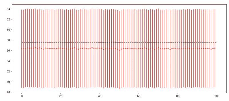
Screenshot 2023-04-14 at 12.55.42 AM.png
 
Physics news on Phys.org
Hi,

To get a feeling for the values, I simplified your expression for P by dividing numerators and denominators by ##x_0## to $$
P = \left ({4/(200\pi)\over y} + {1\over 10}\right )^2 \Bigl(1 - cos(\pi y)\Bigr)$$ where now ##\ y=x/x_0\ ## has a gaussian distribution with average 1 and ##\sigma## 0.1

If there is no error in your expression, P varies from 0.0583 to 0.0545 when ##x## varies from ##180\pi## to ##220\pi##.

Perhaps nothing wrong with all that.

But I have a hard time following
kelly0303 said:
In my simulations I sample x 1000 times and compute P for each of these, then I sum up all the P values, which is basically the number of events I would see in the experiment (0.058 probability x 1000 experiments ~ 58 measured event), call it N. The uncertainty on N, in my simulations, I assume to be ##\sqrt N##.
Isn't ##\sqrt {N\over1000} ## the estimated uncertainty ?

##\ ##
 
##P## is not symmetric wrt ##x = 200 \pi##, but is skewed towards lower values. Normally distributed ##x## centered around ##200 \pi## will thus lead to lower average ##P## than ##P(x = 200\pi)##, so this is normal (pun intended).

Is the equation for ##P## correct? Is it really ##\pi x## in the numerator in the cosine, not simply ##x##?
 
  • Like
Likes   Reactions: hutchphd
1681462125714.png
 
BvU said:
Hi,

To get a feeling for the values, I simplified your expression for P by dividing numerators and denominators by ##x_0## to $$
P = \left ({4/(200\pi)\over y} + {1\over 10}\right )^2 \Bigl(1 - cos(\pi y)\Bigr)$$ where now ##\ y=x/x_0\ ## has a gaussian distribution with average 1 and ##\sigma## 0.1

If there is no error in your expression, P varies from 0.0583 to 0.0545 when ##x## varies from ##180\pi## to ##220\pi##.

Perhaps nothing wrong with all that.

But I have a hard time following

Isn't ##\sqrt {N\over1000} ## the estimated uncertainty ?

##\ ##
I definitely don't know much about statistics, but usually when I was assigning an uncertainty on a given number of counts (for example on a bin in a histogram and assuming more than ~10 counts or so), I was using ##\sqrt{N}## as the statistical uncertainty. So in this case, after 1000 measurements I would have ~58 counts, so I assumed the uncertainty would be directly on the counts that I physically measured i.e. ##\sqrt{58}## and the value of the probability for example would be ~##0.058 \pm \sqrt{58}/1000##. Why would I divide by 1000 under the integral and then once again when moving from counts to actual probability?
 
Test it out: instead of 1000 do 4000 or 9000 and see what happens to the scatter
 
BvU said:
Test it out: instead of 1000 do 4000 or 9000 and see what happens to the scatter
I am attaching below the result for 10000 and 100000 events per experiment. It seems like the more events I have the more I underestimate the uncertainty... Now I am really confused
Screenshot 2023-04-14 at 10.00.46 AM.png
Screenshot 2023-04-14 at 10.00.53 AM.png
 
DrClaude said:
##P## is not symmetric wrt ##x = 200 \pi##, but is skewed towards lower values. Normally distributed ##x## centered around ##200 \pi## will thus lead to lower average ##P## than ##P(x = 200\pi)##, so this is normal (pun intended).

Is the equation for ##P## correct? Is it really ##\pi x## in the numerator in the cosine, not simply ##x##?
But why are the uncertainties so weird, and why they start to underestimate the value as I go to higher N. Also how should I deal with this shift in one direction in practice?

The equation is correct, I need to get ##2## in the ideal case for the term in the second bracket.
 
kelly0303 said:
In my simulations I sample x 1000 times
using some library function ?
 
  • #10
kelly0303 said:
then I sum up all the P values, which is basically the number of events I would see
This is the issue.

You need to not sum up the P values. You need to sample a Bernoulli RV with each P value. In the figure below the blue dots are using the "sum up all the P values" approach, while the orange dots sample a Bernoulli RV with each P value.

random.jpg
 
  • Like
Likes   Reactions: BvU
  • #11
kelly0303 said:
It is a counting experiment where the probability of getting an event after a given trial is given by
Can you explain this ? A probability that depends on a sample value ?

##\ ##
 
  • #12
Dale said:
This is the issue.

You need to not sum up the P values. You need to sample a Bernoulli RV with each P value. In the figure below the blue dots are using the "sum up all the P values" approach, while the orange dots sample a Bernoulli RV with each P value.

View attachment 324884
Thanks a lot! I see, I initially wanted to do that, but it seemed more complicated to implement and I went for the sum. But why are they not equivalent (in the limit of large number of events)?

EDIT: That still seems to underestimate the true value for high number of event. I am attaching below what I am getting for ##10^6## event per point. I am still not sure why this is happening. Shouldn't my uncertainty account for that, even if I might underestimate the true value?

Screenshot 2023-04-14 at 1.14.45 PM.png
 
Last edited:
  • #13
kelly0303 said:
That still seems to underestimate the true value for high number of event.
I am not sure where your “true value” comes in.
 
  • #14
Dale said:
I am not sure where your “true value” comes in.
That is achieved when ##x = x_0##. Basically it would be the value I would measure all the time if I had no uncertainty on ##x##.
 
  • #15
kelly0303 said:
That is achieved when ##x = x_0##. Basically it would be the value I would measure all the time if I had no uncertainty on ##x##.
If you look at ##P## you will see that its range is substantially asymmetric about ##0.058##. It is close to the maximum, so there are very few values of ##x## that produce ##P>0.058## and there are many values of ##x## that produce ##P<0.058##. So the overall result will be naturally biased low.
 
  • #16
Dale said:
If you look at ##P## you will see that its range is substantially asymmetric about ##0.058##. It is close to the maximum, so there are very few values of ##x## that produce ##P>0.058## and there are many values of ##x## that produce ##P<0.058##. So the overall result will be naturally biased low.
I see, but how can I properly estimate the uncertainty such that the result is still consistent with the true value, given the errorbars? Shouldn't that be the case for a properly estimated value? Or how else I should proceed with my analysis given this setup such that I can extract experimentally the correct value i.e. the true probability?
 
  • #17
kelly0303 said:
how else I should proceed with my analysis given this setup such that I can extract experimentally the correct value
You may be able to use a Bayesian approach, although I have never done one quite like this. So I am not certain with the details, but that would be the direction I would go.

Edit: I think maybe a GLM would work.
 
Last edited:
  • #18
Dale said:
You may be able to use a Bayesian approach, although I have never done one quite like this. So I am not certain with the details, but that would be the direction I would go.

Edit: I think maybe a GLM would work.
Thank you! I am still confused about the result I am getting. Why is applying the normal error propagation formula not working in this case? Especially that we have only one variable, so no issues with correlations between variables, I expected that to work. Are there cases where that formula is simply not usable? I assumed that is quite universal.
 
  • #19
kelly0303 said:
Why is applying the normal error propagation formula not working in this case?
Sorry, I missed this. Where did you apply the propagation of uncertainty?

In general, the standard uncertainty propagation formula uses a first order Taylor series approximation. So it will only be exact for a linear function. This problem P is quite nonlinear. Probably you would need at least a second order expansion.
 
Last edited:

Similar threads

  • · Replies 22 ·
Replies
22
Views
2K
  • · Replies 12 ·
Replies
12
Views
3K
  • · Replies 2 ·
Replies
2
Views
2K
  • · Replies 3 ·
Replies
3
Views
3K
  • · Replies 1 ·
Replies
1
Views
2K
  • · Replies 3 ·
Replies
3
Views
2K
  • · Replies 4 ·
Replies
4
Views
2K
  • · Replies 5 ·
Replies
5
Views
2K
  • · Replies 7 ·
Replies
7
Views
2K
  • · Replies 6 ·
Replies
6
Views
2K