MHB Glamour's questions at Yahoo Answers regarding optimization with constraint

[MarkFL]

Here are the questions:

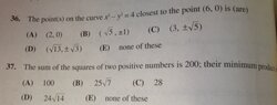
AP Calculus linearization help please?


I don't get this topic so can you guys explain these question as simply as possible? Thanks

View attachment 1900

I have posted a link there to this thread so the OP can view my work.

 

[MarkFL]

Hello Glamour,

36.) We have a point $(x,y)$ which is constrained to line on the curve:

$$x^2-y^2=4$$

Our objective function, that is, what we are seeking to minimize, is the distance between the points $(x,y)$ and $(6,0)$. Now, we may simplify our calculations somewhat if we define our objective function to be the square of this distance. Minimizing the square of the distance will also minimize the distance.

So, our objective function is:

$$f(x,y)=(x-6)^2+y^2$$

Subject to the constraint:

$$g(x,y)=x^2-y^2-4=0$$

First, let's look at a single-variable method. If we solve the constraint for $y^2$, we find:

$$y^2=x^2-4$$

Now, substituting this into our objective function, we get a function of one variable $x$:

$$f(x)=(x-6)^2+x^2-4=x^2-12x+36+x^2-4=2x^2-12x+32=2\left(x^2-6x+16 \right)=2(x+2)(x-8)$$

Pre-Calculus method of optimization:

We observe that because the coefficient of the squared term is positive, this parabolic function opens upwards, thus the vertex will be the global minimum. The axis of symmetry must lie midway between the roots:

$$x=\frac{-2+8}{2}=3$$

Substituting for $x$ into the constraint, we find:

$$y^2=(3)^2-4=5$$

Thus:

$$y=\pm\sqrt{5}$$

And so we conclude the points on the given curve closest to the given point are:

$$\left(3,\pm\sqrt{5} \right)$$

Single variable calculus method of optimization:

Recall we have the objective function:

$$f(x)=2\left(x^2-6x+16 \right)$$

To find the critical value(s), we differentiate with respect to $x$ and equate the result to zero and solve for $x$:

$$f'(x)=2\left(2x-6 \right)=4(x-3)=0\implies x=3$$

Now, we see that the second derivative of $f$ is a positive constant, thus we may conclude the extrema associated with this critical value is the global minimum.

As before, we substitute this critical value into the constraint to obtain the critical points:

$$\left(3,\pm\sqrt{5} \right)$$

Multi-variable method of optimization (Lagrange Multipliers):

Recall our objective function is:

$$f(x,y)=(x-6)^2+y^2$$

Subject to the constraint:

$$g(x,y)=x^2-y^2-4=0$$

This gives rise to the system:

$$2(x-6)=\lambda(2x)$$

$$2y=\lambda(-2y)$$

The second equation implies $\lambda=-1$, and so the first equation becomes:

$$x-6=-x\implies x=3$$

And as before, we substitute this critical value into the constraint to obtain the critical points:

$$\left(3,\pm\sqrt{5} \right)$$

37.) Let's let $x$ and $y$ be the two positive real numbers. Our objective function is their product:

$$f(x,y)=xy$$

And they are subject to the constraint:

$$x^2+y^2=200$$

Now, if we notice that the two variables possesses cyclic symmetry, that is we may exchange them without changing either the objective function or the constraint, then we may conclude immediately that an extremum will occur when $x=y$. Substituting for $y$ into the constraint, we find:

$$x^2+x^2=200$$

$$x^2=100$$

And taking the positive root, we conclude:

$$x=y=10$$

But, if we observe that as either $x$ or $y$ approaches $0$, the other variable must approach $10\sqrt{2}$ and the objective function will then approach zero in either case.

And so we may write:

$$f_{\max}=f(10,10)=10^2=100$$

$$f_{\min}=\lim_{x\to0}(xy)=0$$

However, let's explore how to work this without appealing to cyclic symmetry.

If we solve the constraint for $y$, taking the positive root, we find:

$$y=\sqrt{200-x^2}$$

Substituting this into our objective function, we find:

$$f(x)=x\sqrt{200-x^2}$$

Differentiating with respect to $x$ (using the Product Rule) and equating the result to zero, we find:

$$f'(x)=x\left(\frac{-2x}{2\sqrt{200-x^2}} \right)+(1)\sqrt{200-x^2}=\frac{2\left(100-x^2 \right)}{\sqrt{200-x^2}}=0$$

Now, we observe that the positive root of the denominator is an end-points of the objective function's domain, which is $0<x\le10\sqrt{2}$ and the (positive) root of the numerator is within the domain, so we have 3 critical values to check:

$$f(0)=0$$

$$f(10)=100$$

$$f\left(10\sqrt{2} \right)=0$$

Based on this, we may conclude:

$$f_{\max}=100$$

$$f_{\min}=0$$

Now, let's look at Lagrange multipliers. We have the objective function:

$$f(x,y)=xy$$

Subject to the constraint:

$$g(x,y)=x^2+y^2-200=0$$

Thus, we obtain the system:

$$y=\lambda(2x)$$

$$x=\lambda(2y)$$

This implies:

$$y^2=x^2$$

Substituting this into the constraint, we find:

$$x^2=100$$

And taking the positive root, we obtain

$$x=y=10$$

Now, as in the other methods we explored, we need to look at the end-points of the domain, to find the above critical point $(x,y)=(10,10)$ is at the global maximum, and the end-point values give the global minimum. As so, as before, we then find:

$$f_{\max}=100$$

$$f_{\min}=0$$