JD_PM
- 1,125
- 156
- TL;DR
- I am aimed at overlapping the plots for the speed distribution over the vertical width profile (which is 0.015 m long; highlighted in red) for two downstream, horizontal distances [w.r.t. the orifice]: 0.01 m and 0.03 m.
How to modify my code such that it swaps all row data?
I am studying a flow going through an orifice.
I am aimed at overlapping the plots for the speed distribution over the vertical width profile (which is 0.015 m long; highlighted in red) for two downstream, horizontal distances [w.r.t. the orifice]: 0.01 m and 0.03 m.

The result should look as follows (the highest peak corresponds to 0.01m width profile)
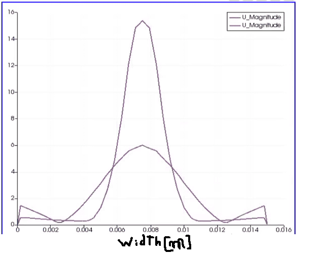
I have the data for both downstream distances (in csv format, here you can find it https://drive.google.com/drive/folders/1CgeDuCahVZvLXXkNkGWlPg8lSGyurmI3).
Let me create two tables, first related to 0.01m data and second to 0.03 m. For the sake of simplicity I only include three row data. The columns labeled - contain irrelevant data for this particular problem.
0.01m data
0.03m data
Let's draw our attention to how to code this in MATLAB. The algorithm I have in mind is:
0) Optimize the given table: eliminate first and last rows (the velocity there is zero due to no-slip condition on the walls)
1) Read the velocity data from the csv table and compute the speed ##U = \sqrt{U_0^2 + U_1^2 + U_2^2}## for each data row.
2) Store the speed and width values in variables.
3) Repeat 2) and 3) for the other csv file.
4) Ready to plot.
I managed to write a code that works for the three-rows-of-data tables above
The issue I have is that I do not see how to write a code that does it for the 1000 rows. I guess there has to be a way of automatizing the whole process...
I am quite sure the code can be written more efficiently (it's my first MATLAB code ever!), so please feel to add suggestions :)
Thank you!
PS: Shout out to the Moderation Staff for asking me to write more details!
I am aimed at overlapping the plots for the speed distribution over the vertical width profile (which is 0.015 m long; highlighted in red) for two downstream, horizontal distances [w.r.t. the orifice]: 0.01 m and 0.03 m.
The result should look as follows (the highest peak corresponds to 0.01m width profile)
I have the data for both downstream distances (in csv format, here you can find it https://drive.google.com/drive/folders/1CgeDuCahVZvLXXkNkGWlPg8lSGyurmI3).
Let me create two tables, first related to 0.01m data and second to 0.03 m. For the sake of simplicity I only include three row data. The columns labeled - contain irrelevant data for this particular problem.
0.01m data
| U0 | U1 | U2 | - | - | X | Y | Z |
| -0.044326 | 3.0829e-05 | 0.0016394 | 1 | 1.5e-05 | 0.01 | 0 | -0.007485 |
| -0.088655 | 6.1659e-05 | 0.003279 | 1 | 3e-05 | 0.01 | 0 | -0.00747 |
| -0.13298 | 9.2489e-05 | 0.0049184 | 1 | 4.5e-05 | 0.01 | 0 | -0.007455 |
0.03m data
| U0 | U1 | U2 | - | - | X | Y | Z |
| -0.11972 | -0.00036133 | -0.0012355 | 1 | 1.5e-05 | 0.03 | 0 | -0.007485 |
| -0.23945 | -0.00072269 | -0.002471 | 1 | 3e-05 | 0.03 | 0 | -0.00747 |
| -0.35918 | -0.001084 | -0.0037066 | 1 | 5e-05 | 0.03 | 0 | -0.007455 |
0) Optimize the given table: eliminate first and last rows (the velocity there is zero due to no-slip condition on the walls)
1) Read the velocity data from the csv table and compute the speed ##U = \sqrt{U_0^2 + U_1^2 + U_2^2}## for each data row.
2) Store the speed and width values in variables.
3) Repeat 2) and 3) for the other csv file.
4) Ready to plot.
I managed to write a code that works for the three-rows-of-data tables above
Matlab:
Ai = readtable("sampleData10mm.csv"); %step 0)
A = Ai(2:1000,:); %step 0)
fComr1 = A{1:1,"U_0"}; %step 1)
sComr1 = A{1:1,"U_1"}; %step 1)
tComr1 = A{1:1,"U_2"}; %step 1)
fComr2 = A{2:2,"U_0"}; %step 1)
sComr2 = A{2:2,"U_1"}; %step 1)
tComr2 = A{2:2,"U_2"}; %step 1)
fComr3 = A{3:3,"U_0"}; %step 1)
sComr3 = A{3:3,"U_1"}; %step 1)
tComr3 = A{3:3,"U_2"}; %step 1)

Ur1 = sqrt(fComr1^2 + sComr1^2 + tComr1^2); %step 1)
Ur2 = sqrt(fComr2^2 + sComr2^2 + tComr2^2); %step 1)
Ur3 = sqrt(fComr3^2 + sComr3^2 + tComr3^2); %step 1)

speed = [0;Ur1;Ur2;Ur3]; %step 2)
width = [0;A{1:1,"Points_2"}+0.0075;A{2:2,"Points_2"}+0.0075;A{3:3,"Points_2"}+0.0075]; %step 2); Note I added +0.0075 because we want to have data from 0 to 0.016 mm in the x axis

Bi = readtable("sampleData30mm.csv"); %step 3)
B = Bi(2:1000,:); %step 3)
fComr1_30mm = B{1:1,"U_0"};  %step 3)
sComr1_30mm = B{1:1,"U_1"};  %step 3)
tComr1_30mm = B{1:1,"U_2"};  %step 3)
fComr2_30mm = B{2:2,"U_0"};  %step 3)
sComr2_30mm = B{2:2,"U_1"};  %step 3)
tComr2_30mm = B{2:2,"U_2"};  %step 3)
fComr3_30mm = B{3:3,"U_0"};  %step 3)
sComr3_30mm = B{3:3,"U_1"};  %step 3)
tComr3_30mm = B{3:3,"U_2"};  %step 3)
Ur1_30mm = sqrt(fComr1_30mm^2 + sComr1_30mm^2 + tComr1_30mm^2); %step 3)
Ur2_30mm = sqrt(fComr2_30mm^2 + sComr2_30mm^2 + tComr2_30mm^2); %step 3)
Ur3_30mm = sqrt(fComr3_30mm^2 + sComr3_30mm^2 + tComr3_30mm^2); %step 3)
speed_30mm = [0;Ur1_30mm;Ur2_30mm;Ur3_30mm]; %step 3)
width_30mm = [0;B{1:1,"Points_2"}+0.0075;B{2:2,"Points_2"}+0.0075;B{3:3,"Points_2"}+0.0075]; %step 3)

figure %step 4)
plot(width,width_30mm,speed,speed_30mm) %step 4)
legend({'0.01 m', '0.03 m'},'Location','northwest') %step 4)
xlabel('width [m]') %step 4)
ylabel('U magnitude [m/s]') %step 4)
axis square; %step 4)
grid on; %step 4)
The issue I have is that I do not see how to write a code that does it for the 1000 rows. I guess there has to be a way of automatizing the whole process...
I am quite sure the code can be written more efficiently (it's my first MATLAB code ever!), so please feel to add suggestions :)
Thank you!
PS: Shout out to the Moderation Staff for asking me to write more details!