I Is there a way to calculate expected value from probabilistic data?

[Feynstein100]

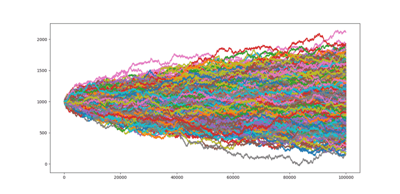
So I ran a python simulation of 1,000 games of toss (50/50 odds) where each game consists of 100,000 consecutive flips. The result was this:

1000 is our starting balance and as expected, there's a nice normal distribution around it. I also calculated the average value after all the games and it was around 1000, again, as expected.

However, then it occurred to me that the expected profit/loss is zero because our graph here represents all possibilities (almost but it's a representative sample so bear with me) and the graph is symmetric about the starting balance i.e. there are just as many outcomes above the starting value as there are under it. Hence, on average, there's no gain/loss.

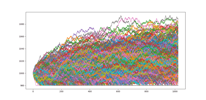
So I thought, what if that weren't true? What if we made the graph asymmetric? If we quit once we reached a balance of, say, 980, the graph would look something like this:

Idk if you guys are familiar with daytrading terms but in case you aren't, this is called a stop-loss, i.e. a thing that prevents you from losing more money than the level you set it at. Anyway, since this graph is clearly asymmetric, I expected more outcomes to be above 1000 than below it. This should've led to a clear profit over the long run. And yet, even when I did 100,000 flips with the stop loss, the average outcome was still around 1000. I'm at a loss as to why that happened. From a purely geometrical point of view, there should've been a net profit.

The graph seems to be following a y = sqrt(x) curve both above and below the starting balance. I assumed the profit/loss would simply be the area under the curves. Profit for the part above 1000 and loss for the part below 1000. Without the stop-loss, these two areas would be equal and cancel each other out, thus no net profit/loss. But with the lower area now restricted because of the stop loss, shouldn't there be more area above and hence a profit? What am I missing here? Is it perhaps incorrect to calculate profit/loss this way?

 

[Office_Shredder]

That picture has a *lot* of lines that hit 980 and then flatline. So your distribution of final values is not normal, and has a huge spike at 980.

You just can't see it in your visualization.

 

[Feynstein100]

That picture has a *lot* of lines that hit 980 and then flatline. So your distribution of final values is not normal, and has a huge spike at 980.

You just can't see it in your visualization.

I didn't realize that. Thanks for your helpful reply. I have a further question. What if we instead made the stop-loss inclined and parallel to the upper boundary of the curve, which represents the most favourable outcome, I think? That way, there won't be a huge spike at 980, it will keep increasing with the no. of flips. That should lead to a profit eventually, right?

 

[Office_Shredder]

I don't know what you mean by upper boundary of the curve. If your stop loss is over 1000 it will trigger before you get to take your first step.

In general a stop loss cannot increase your expected value. The total expected value is the sum of the expected values of each step, and you aren't doing anything to change the expected value of any step. You just reduce the variance.

 

[Feynstein100]

I don't know what you mean by upper boundary of the curve. If your stop loss is over 1000 it will trigger before you get to take your first step.

In general a stop loss cannot increase your expected value. The total expected value is the sum of the expected values of each step, and you aren't doing anything to change the expected value of any step. You just reduce the variance.

This is what I had in mind: an inclined stop-loss instead of a horizontal one. I somehow feel like this should lead to some change. Maybe it's my intuition from quantum mechanics but I kind of see a similar pattern here. A particle takes all possible paths until it's observed, right? But if we restrict some of those paths, we should get something like the Casimir effect? Idk

 

[BWV]

So I ran a python simulation of 1,000 games of toss (50/50 odds) where each game consists of 100,000 consecutive flips. The result was this:
View attachment 314169
1000 is our starting balance and as expected, there's a nice normal distribution around it. I also calculated the average value after all the games and it was around 1000, again, as expected.

However, then it occurred to me that the expected profit/loss is zero because our graph here represents all possibilities (almost but it's a representative sample so bear with me) and the graph is symmetric about the starting balance i.e. there are just as many outcomes above the starting value as there are under it. Hence, on average, there's no gain/loss.

So I thought, what if that weren't true? What if we made the graph asymmetric? If we quit once we reached a balance of, say, 980, the graph would look something like this:
View attachment 314170
Idk if you guys are familiar with daytrading terms but in case you aren't, this is called a stop-loss, i.e. a thing that prevents you from losing more money than the level you set it at. Anyway, since this graph is clearly asymmetric, I expected more outcomes to be above 1000 than below it. This should've led to a clear profit over the long run. And yet, even when I did 100,000 flips with the stop loss, the average outcome was still around 1000. I'm at a loss as to why that happened. From a purely geometrical point of view, there should've been a net profit.

The graph seems to be following a y = sqrt(x) curve both above and below the starting balance. I assumed the profit/loss would simply be the area under the curves. Profit for the part above 1000 and loss for the part below 1000. Without the stop-loss, these two areas would be equal and cancel each other out, thus no net profit/loss. But with the lower area now restricted because of the stop loss, shouldn't there be more area above and hence a profit? What am I missing here? Is it perhaps incorrect to calculate profit/loss this way?

the graph follows a curve on the order of sqrt(x) because the variance of this model is p(1-p) = 0.25, as the standard deviation is the square root of the variance, the spread of outcomes increases with the square root of x, so the standard deviation at x=1000 is 500 and what you see at that point, as expected, is almost all the outcomes within 2 standard deviations (+-1000)

The coin flip is a martingale, meaning the expected value at x equals the value at x, nothing you can do with stop losses changes this. Think about it - why should it be possible to change a bet with a zero expected gain to a positive one with some trading rule? people peddle this BS all the time in financial markets, but it does not work. Stop losses, for example, do not add value to trading stocks

 

[BWV]

If you are interested in calculating an expectation of some function of this process, then you get into option pricing. For example, say I offer to let you play this game with a guarantee that you cannot lose more than 10% of your initial stake, what is the expected value (or fair value you would pay) for that?

 

[Vanadium 50]

In general a stop loss cannot increase your expected value.

@Feynstein100 ,do you understand why?

This protects you from when you are at 980 and eventually reach 960. But what happens when you are at 980 and it will eventually reach 1020?

 

[Feynstein100]

@Feynstein100 ,do you understand why?

This protects you from when you are at 980 and eventually reach 960. But what happens when you are at 980 and it will eventually reach 1020?

I still don't get it. Let me put it this way: With a stop-loss, you can theoretically make infinite money but you can only lose a certain amount. Over time, shouldn't this lead to a net profit? What's wrong with this line of thinking?

 

[Feynstein100]

the graph follows a curve on the order of sqrt(x) because the variance of this model is p(1-p) = 0.25, as the standard deviation is the square root of the variance

Wow, I didn't know that. Thanks so much! This explains a lot. With this knowledge, perhaps I can phrase my argument better. Apparently all a stop-loss does is reduce the variance/standard deviation and my postulate is that the expected value is a function of standard deviation.
If that is true, when the standard deviation changes, the expected value must change as well.
I see two possible alternatives:
1. The expected value is NOT a function of standard deviation and thus changes in the latter have no influence on the former.
2. The expected value is indeed a function of standard deviation but NOT ONLY standard deviation. There are also other variables at play and when the s.d. changes, the other variables change in such a way that the expected value is unchanged.
One of these 3 possibilities has to be true, right? So I guess the question is, which one is it?

 

[Hornbein]

The expected value is not a function of standard deviation.

 

[Hornbein]

I still don't get it. Let me put it this way: With a stop-loss, you can theoretically make infinite money but you can only lose a certain amount. Over time, shouldn't this lead to a net profit? What's wrong with this line of thinking?

Whenever you sell at a loss, you guarantee a loss. There is no longer a possibility of doing better.

You have probability zero of making infinite money.

But to me the best explanation is that the math tells you so. Or you can do a computer simulation that will tell you so. There is no trading rule that will increase your expectation. It seems to me the fiscal equivalent of a perpetual motion machine.

Also common are trading rules that produce many small gains and a few big losses. Such schemes were responsible for the bankruptcy of Long Term Capital Management and others.

A federal government that will cover those big losses due to the "too big to fail" doctrine will however increase one's expectation.

 

[BWV]

There is no trading rule that will increase your expectation. It seems to me the fiscal equivalent of a perpetual motion machine.

Actually there is one (at least mathematically) - the martingale (the origin of the statistical term), where you double the bet after each loss. Problem is it requires an infinite bankroll

https://en.m.wikipedia.org/wiki/Martingale_(betting_system)

 

[Hornbein]

Actually there is one (at least mathematically) - the martingale (the origin of the statistical term), where you double the bet after each loss. Problem is it requires an infinite bankroll

https://en.m.wikipedia.org/wiki/Martingale_(betting_system)

As my professor said, "nobody in his right mind would bet everything he had to play this game."

 

[BWV]

The other interesting variant is the St Petersburg paradox, a game with an infinite expectation that no one would pay more than about $40 to play

 

[Feynstein100]

The expected value is not a function of standard deviation.

@BWV Could you confirm this?

 

[BWV]

@BWV Could you confirm this?

Correct the variance / standard deviation does not impact the expectation - say instead of doubling / losing your money the payoff is 2x, so on a $1 bet you win/lose $2. The expectation is still 0.5(2)+0.5*(-2) = 0. But the standard deviation has doubled:
var=E(X^2)-E(X)^2. = 4 so the standard deviation is 2

 

[jbriggs444]

I didn't realize that. Thanks for your helpful reply. I have a further question. What if we instead made the stop-loss inclined and parallel to the upper boundary of the curve, which represents the most favourable outcome, I think? That way, there won't be a huge spike at 980, it will keep increasing with the no. of flips. That should lead to a profit eventually, right?

There is no way to sum up a [possibly truncated based on prior results] finite series of bets, each with expectation zero and wind up with anything but an expectation of zero.

 

[pbuk]

@Feynstein100 you don't need to do any maths to see that the stop loss does not change the expected value if returns are symmetrical, you just need to look at the symmetry. Think about the expected value of the investments you sell at 980.

Once you have thought this through, see if you can predict what a stop loss will do in a rising market, then run a simulation.

 

[Hornbein]

Pro poker players often do things to reduce standard deviation. This lessens their vulnerability to a run of bad luck, which they say WILL happen anyway. I think these bets also reduce their expectation, but they say it's worth it.

 

[Feynstein100]

It seems to me the fiscal equivalent of a perpetual motion machine.

I noticed that too. It's similar to the conservation of energy. The expectation value is always constant, no matter what you do. However, isn't conservation of energy result from time symmetry, as proved by Nöther? And in the scale of GR, where time symmetry is no longer valid, conservation of energy is no longer valid either?
Perhaps we could do something similar to expectation value. If it is indeed conserved, does that mean there's a corresponding symmetry somewhere?

 

[pbuk]

Perhaps we could do something similar to expectation value. If it is indeed conserved, does that mean there's a corresponding symmetry somewhere?

Yes, and if you follow my suggestions in post #19 you should be able to see where.

 

[BWV]

Also in the real world, stock prices can gap down with stop losses providing no protection. NFLX, for example, closed at $349 on April 19 then opened at $245 the following morning

 

[FactChecker]

And yet, even when I did 100,000 flips with the stop loss, the average outcome was still around 1000. I'm at a loss as to why that happened. From a purely geometrical point of view, there should've been a net profit.
...
But with the lower area now restricted because of the stop loss, shouldn't there be more area above and hence a profit? What am I missing here? Is it perhaps incorrect to calculate profit/loss this way?

CORRECTION: THIS IS WRONG: Yes, it looks like the average profit should be significantly higher. I don't see any description of how you are calculating the average profit, but I assume that it is a simple part of the simulation. IMO, there must be an error in it.
Is it possible that the graph is deceptive and the part that is modified is a much smaller percentage than it appears to be?
Thanks @Office_Shredder ! I stand corrected. My intuition misguided me.
The way I see this now is that any simulation that was stopped by a stop-loss at 980 would have an expected result of 980 if it was allowed to continue. So the expected result does not change by stopping them.

 

[Office_Shredder]

The average profit should not be higher @FactChecker the graph they put in the original post is a terrible way of visualizing what is going on.

 

[jbriggs444]

Crude drawing to reprise what @Office_Shredder pointed out in #2. (Very crude).

You would be integrating outcome times probability density. Plus a contribution for the discrete probability spike at the stop loss point.

That spike is not a probability density. It is a probability.

I think that the stop loss shifts the "mode" (the high point) on the probability density function (PDF) slightly to the right. But it leaves the expected value unchanged due to the contribution of the new spike.

 

[FactChecker]

The average profit should not be higher @FactChecker the graph they put in the original post is a terrible way of visualizing what is going on.

Thanks! I stand corrected. My intuition misguided me.
The way I see this now is that any simulation that was stopped by a stop-loss at 980 would have an expected result of 980 if it was allowed to continue. So the expected result does not change by stopping them at 980.

 

[BWV]

was looking and, not suprisingly, there is a theorem about this that states the expected value of a martingale given a stopping time is equal to the total expectation

https://en.wikipedia.org/wiki/Optional_stopping_theorem

https://math.dartmouth.edu/~pw/math100w13/lalonde.pdf

 

[pbuk]

Thanks! I stand corrected. My intuition misguided me.
The way I see this now is that any simulation that was stopped by a stop-loss at 980 would have an expected result of 980 if it was allowed to continue. So the expected result does not change by stopping them at 980.

Er, yes. Am I on mute?

 

[FactChecker]

Er, yes. Am I on mute?

Sorry, I saw your post #19 but I missed the point of it.

 

[Office_Shredder]

Once you understand that adding these stops doesn't change your expected value, you can do a very cool computation.

Suppose I sell if it goes down to 980, or up to 1060. What's the probability it hits 980 first?

Hint: if the probability is p, compute your expected value. What does it have to equal?

 

[Feynstein100]

The average profit should not be higher @FactChecker the graph they put in the original post is a terrible way of visualizing what is going on.

That's a bit strong lol. Graphs are useful as long as you know what they represent. My original graph was meant to represent the possible paths followed by a game of consecutive coin flips. It's literally what's going on. It was never meant to represent the number of heads and tails you got. Although, the other graph sounds interesting too. I'll see if I can change my code to draw that graph too.

 

[Feynstein100]

Once you understand that adding these stops doesn't change your expected value, you can do a very cool computation.

Suppose I sell if it goes down to 980, or up to 1060. What's the probability it hits 980 first?

Hint: if the probability is p, compute your expected value. What does it have to equal?

Hmm that's an interesting question. My intuition says that both outcomes are equally likely i.e. p = 1-p = 0.5
So, the expectation value would be
1020 * 0.5 - 980 * 0.5 = 20
Which shouldn't be possible because I feel like the expectation value should still be zero. There must be an error here somewhere
Edit: changed 1060 to 1020 because 1060 isn't equally likely as 980, 1020 is.
Edit2: My formula for expectation value was wrong. The actual formula is just the sum of each outcome multiplied by its probability. Which gives us
1020 * 0.5 + 980 * 0.5 = 1000
As expected

 

[jbriggs444]

Hmm that's an interesting question. My intuition says that both outcomes are equally likely i.e. p = 1-p = 0.5
So, the expectation value would be
1020 * 0.5 - 980 * 0.5 = 20
Which shouldn't be possible because I feel like the expectation value should still be zero. There must be an error here somewhere
Edit: changed 1060 to 1020 because 1060 isn't equally likely as 980, 1020 is.

You are subtracting when you should be adding.

 

[Feynstein100]

You are subtracting when you should be adding.

Damn, dude. You beat me to the punch by a millisecond

 

[pbuk]

1020 * 0.5 + 980 * 0.5 = 1000

Yes but that is trivial, what @Office_Shredder was asking is more interesting: 1060 * ? + 980 * ? = ?

 

[Feynstein100]

Yes but that is trivial, what @Office_Shredder was asking is more interesting: 1060 * ? + 980 * ? = ?

Eh idk. In the end it should still come out to 1000. 1060 may be a higher value but it's less likely to happen than 980. These two factors balance each other out and the result is still 1000.

 

[Feynstein100]

The expected value is not a function of standard deviation.

@BWV
Turns out, there's more to this. I took this from Wikipedia:

Here, mu is the mean/expected value. So while mu isn't a function of sigma, the two do interact with each other. It's just that when you change sigma, you also change the probability and the resulting data points, in just such a way that mu remains unchanged. My hunch was correct, in a sense

 

[Office_Shredder]

This is a general statement that if you want to compute the standard deviation, you have to subtract the mean out. This is actually what prevents them from usually being related - if you adjust the mean by adding some quantity to every outcome, that doesn't affect the standard deviation at all.

 

[jbriggs444]

Eh idk. In the end it should still come out to 1000. 1060 may be a higher value but it's less likely to happen than 980. These two factors balance each other out and the result is still 1000.

We are trying to solve for the probability ratio. I do not know if @Office_Shredder has a particular approach in mind, but here is how I would attack it.

Let $p$ be the probability of first hitting 980. Then $1-p$ is the probability of first hitting 1060. We are in an infinite random walk (as I recall), so the probability of never hitting either is obviously zero.

We know that the mean of the infinite random walk needs to be 1000 because that is the starting point and every step is unbiased. So we write down an equation: $980 p + 1060(1-p) = 1000$

Now we just have to solve for p. Easy algebra. Then write down the ratio in the form $p:1-p$.

If intuition serves, we should find that the sides of the ratio are in inverse proportion to each side's deviation from the mean. The deviations are 20:60 so the probability ratio will be 3:1.

[It feels like there should be some more directly compelling algebra if I'd made a better choice of variables. But I will not change horses mid-stream]

Let us see whether the algebra bears this out...

$980p + 1060 (1-p) = 1000$
$(980 - 1060)p + 1060 = 1000$
$-80p = -60$
$p = \frac{3}{4}$
$1-p = \frac{1}{4}$

Ratio = 3:1

Bingo.

 

[Feynstein100]

We are trying to solve for the probability ratio. I do not know if @Office_Shredder has a particular approach in mind, but here is how I would attack it.

Let $p$ be the probability of first hitting 980. Then $1-p$ is the probability of first hitting 1060. We are in an infinite random walk (as I recall), so the probability of never hitting either is obviously zero.

We know that the mean of the infinite random walk needs to be 1000 because that is the starting point and every step is unbiased. So we write down an equation: $980 p + 1060(1-p) = 1000$

Now we just have to solve for p. Easy algebra. Then write down the ratio in the form $p:1-p$.

If intuition serves, we should find that the sides of the ratio are in inverse proportion to each side's deviation from the mean. The deviations are 20:60 so the probability ratio will be 3:1.

[It feels like there should be some more directly compelling algebra if I'd made a better choice of variables. But I will not change horses mid-stream]

Let us see whether the algebra bears this out...

$980p + 1060 (1-p) = 1000$
$(980 - 1060)p + 1060 = 1000$
$-80p = -60$
$p = \frac{3}{4}$
$1-p = \frac{1}{4}$

Ratio = 3:1

Bingo.

Oh.....kay? Don't get me wrong. That was quite interesting but I was kinda expecting a cheat or a workaround of some kind As it stands, we're right where we started. Conservation of expectation value shall not be violated.

 

[jbriggs444]

Oh.....kay? Don't get me wrong. That was quite interesting but I was kinda expecting a cheat or a workaround of some kind As it stands, we're right where we started. Conservation of expectation value shall not be violated.

Right. Re-read #31. @Office_Shredder is not trying to prove conservation of expected value. He is trying to use the principle of conservation of expected value to reach a conclusion about the probability of hitting the stop points.

Conservation of expected value is on pretty solid ground (for a reasonable set of assumptions). I took the assumption to be a starting bankroll of 1000 quatloos and a series of unbiased coin flips that result in a gain or loss of 1 quatloo with probability 0.5 each (an unbiased infinite random walk) with stop points at 980 quatloos or 1060 quatloos.

 

[Feynstein100]

This is a general statement that if you want to compute the standard deviation, you have to subtract the mean out. This is actually what prevents them from usually being related - if you adjust the mean by adding some quantity to every outcome, that doesn't affect the standard deviation at all.

Ah okay. It's more nuanced than I'd anticipated. Btw the equations don't tell us how they change when we use a stop-loss to change sigma. I mean, I kind of discovered it empirically from my python code but is there a way to see it happen mathematically? A proof or something? Idk. I tried to read the proof of the optional stopping theorem but it was beyond me. Way too abstract lol.

 

[Feynstein100]

Right. Re-read #31. @Office_Shredder is not trying to prove conservation of expected value. He is trying to use the principle of conservation of expected value to reach a conclusion about the probability of hitting the stop points.

Oh. My bad. I thought we were trying to find a workaround/loophole

 

[jbriggs444]

Oh. My bad. I thought we were trying to find a workaround/loophole

There are none unless you decide to allow shenanigans such as unbounded bets. e.g. a Martingale scheme. There was a reference upthread to a relevant theorem.

 

[Hornbein]

The sum of the expectations is the expectation of the sum. Each bet has zero expectation. So the expectation of the sum of those bets is zero. It doesn't matter how you decide whether or not to make those bets.

 

[BWV]

Is conservation of expected value is just another way of stating the process is a Martingale - defined as E(T1)=E(Tn) for all n. Not every process would have this attribute

 

[BWV]

@BWV
Turns out, there's more to this. I took this from Wikipedia:
View attachment 314407
Here, mu is the mean/expected value. So while mu isn't a function of sigma, the two do interact with each other. It's just that when you change sigma, you also change the probability and the resulting data points, in just such a way that mu remains unchanged. My hunch was correct, in a sense

If you want to see where the variance influence the mean, change the payoff to + or - 10% of the previous value then compare to another where it is + or - 50% (does not change the mean but the expectation relates to the difference between the mean and median: at + or - 50% you almost surely will go broke if you play long enough even though the expected gain/loss is zero

 

[Feynstein100]

Is conservation of expected value is just another way of stating the process is a Martingale - defined as E(T1)=E(Tn) for all n. Not every process would have this attribute

Sorry I didn't get that. Could you explain it again?

 

[jbriggs444]

Sorry I didn't get that. Could you explain it again?

Does this wiki page make it any more clear?