ME's question at Yahoo Answers regarding pursuit curve

[MarkFL]

Here is the question:

How do you solve this really hard calculus question?

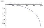
Ship A and ship B start 100 km apart from each other (oriented so that a horizontal line will pass through both). As time passes, ship A moves straight down at a speed of 10 km/hr. Ship B moves towards ship A at all times so that the slope at which ship B is moving on is always one who's line points directly towards ship A at that instance. Ship B is always moving at 12 km/hr. How do I find the function which represents the path which ship B moves along? The function may have as many variables in it as you want. I just need to know the function, and how to find it.

Here is a link to the question:

How do you solve this really hard calculus question? - Yahoo! Answers

I have posted a link there to this topic so the OP can find my response.

 

[MarkFL]

Hello ME,

An interesting geometric model arises when one tries to determine the path of a pursuer chasing its "prey." This path is called a curve of pursuit. These problems were analyzed using methods of calculus circa 1760 (more than two centuries after Leonardo da Vinci had considered them).

The simplest problem is to find the curve along which a vessel moves when pursuing another vessel that flees along a straight line, assuming the speeds of the two vessels are constant.

Let's assume ship $B$, traveling at speed $\beta$, is pursuing ship $A$, which is traveling at speed $\alpha$. In addition, assume that ship $B$ begins (at time $t=0$) at the origin and pursues ship $A$, which begins at the point $(b,0)$ where $0<b$ and travels down the line $x=b$.

After $t$ hours, ship $B$ is located at the point $P(x,y)$, and ship $A$ is located at the point $Q(b,-\alpha t)$. The goal is then to describe the locus of points $P$, that is, to find $y$ as a function of $x$.

(a) Since ship $B$ is pursuing ship $A$, then at time $t$, ship $B$ must be heading right at ship $A$. That is, the tangent line to the curve of pursuit at $P$ must pass through the point $Q$. Using the point-slope formula, this implies:

\(\displaystyle y+\alpha t=\frac{dy}{dx}(x-b)\)

(1) \(\displaystyle \frac{dy}{dx}=\frac{y+\alpha t}{x-b}\)

(b) Since we know the speed at which ship $B$ is traveling, we know the distance it travels is $\beta t$. This distance is also the length of the pursuit curve from $(0,0)$ to $(x,y)$. Using the arc length formula from calculus, we find that:

(2) \(\displaystyle \beta t=\int_0^x \sqrt{1+\left(y'(u) \right)^2}\,du\)

Solving for $t$ in equations (1) and (2), we find that:

(3) \(\displaystyle (x-b)\frac{dy}{dx}-y=\frac{\alpha}{\beta}\int_0^x \sqrt{1+\left(y'(u) \right)^2}\,du\)

(c) Differentiating both sides of (3) with respect to $x$, we find:

\(\displaystyle \left((x-b)\frac{d^2y}{dx^2}+\frac{dy}{dx} \right)-\frac{dy}{dx}=\frac{\alpha}{\beta}\sqrt{1+\left( \frac{dy}{dx} \right)^2}\)

Letting \(\displaystyle \omega=\frac{dy}{dx}\) we obtain the first order IVP:

\(\displaystyle (x-b)\frac{d\omega}{dx}=\frac{\alpha}{\beta}\sqrt{1+ \omega^2}\) where \(\displaystyle \omega(0)=0\)

(d) Using separation of variables, and switching the dummy variables of integration so that we may use the boundaries as the limits, we find:

\(\displaystyle \int_0^{\omega}\frac{1}{\sqrt{1+u^2}}\,du= \frac{\alpha}{\beta}\int_0^x\frac{1}{v-b}\,dv\)

Integrating, we find:

\(\displaystyle \left[\ln|u+\sqrt{1+u^2}| \right]_0^{\omega}=\frac{\alpha}{\beta}\left[\ln|v-b| \right]_0^x\)

\(\displaystyle \ln|\omega+\sqrt{1+\omega^2}|=\ln\left|\left(1-\frac{x}{b} \right)^{\frac{\alpha}{\beta}} \right|\)

Since \(\displaystyle -\infty\le \omega<0\) and \(\displaystyle 0<1-\frac{x}{b}\) we may state:

\(\displaystyle \omega+\sqrt{1+\omega^2}=-\left(1-\frac{x}{b} \right)^{\frac{\alpha}{\beta}}\)

\(\displaystyle \left(\sqrt{1+\omega^2} \right)^2=\left(\left(1-\frac{x}{b} \right)^{\frac{\alpha}{\beta}}+\omega \right)^2\)

\(\displaystyle 1+\omega^2=\left(1-\frac{x}{b} \right)^{\frac{2\alpha}{\beta}}+2\omega\left(1-\frac{x}{b} \right)^{\frac{\alpha}{\beta}}+\omega^2\)

\(\displaystyle 2\omega\left(1-\frac{x}{b} \right)^{\frac{\alpha}{\beta}}=1-\left(1-\frac{x}{b} \right)^{\frac{2\alpha}{\beta}}\)

Back-substituting for $\omega$, we have the IVP:

\(\displaystyle \frac{dy}{dx}=\frac{1}{2}\left(\left(1-\frac{x}{b} \right)^{-\frac{\alpha}{\beta}}-\left(1-\frac{x}{b} \right)^{\frac{\alpha}{\beta}} \right)\) where \(\displaystyle y(0)=0\)

Switching the dummy variables of integration so we can use the boundaries, we have:

\(\displaystyle \int_0^y\,du=\frac{1}{2}\int_0^x\left(1-\frac{v}{b} \right)^{-\frac{\alpha}{\beta}}-\left(1-\frac{v}{b} \right)^{\frac{\alpha}{\beta}}\,dv\)

\(\displaystyle _0^y=\frac{b}{2}\left[\frac{\left(1+\frac{v}{b} \right)^{1+\frac{\alpha}{\beta}}}{1+\frac{\alpha}{\beta}}-\frac{\left(1-\frac{v}{b} \right)^{1-\frac{\alpha}{\beta}}}{1-\frac{\alpha}{\beta}} \right]_0^x\)

After simplifying, we obtain:

\(\displaystyle y=\frac{b\beta}{2(\alpha^2-\beta^2)}\left((\beta-\alpha)\left(1-\frac{x}{b} \right)^{\frac{\beta+\alpha}{\beta}}-(\beta+\alpha)\left(1-\frac{x}{b} \right)^{\frac{\beta-\alpha}{\beta}}+2\alpha \right)\)

Plugging in the given data $b=100,\,\alpha=10,\,\beta=12$ we find:

\(\displaystyle y=-\frac{300}{11}\left(\left(1-\frac{x}{100} \right)^{\frac{11}{6}}-11\left(1-\frac{x}{100} \right)^{\frac{1}{6}}+10 \right)\)

Here is a plot of the pursuit curve, i.e., the path of ship B:

https://www.physicsforums.com/attachments/822._xfImport

To ME and any other guests viewing this topic, I invite and encourage you to post other calculus questions here in our http://www.mathhelpboards.com/f10/ forum.

Best Regards,

Mark.