Frank Einstein
- 166
- 1
Hello everyone. I am trying to construct a functioning version of randomfields (specifically 2D_karhunen_loeve_identification_example.py) in Matlab. For that, I have to calculate the Karhunen-Loève expansion of 2D data, since this is what it says in the documentation. I also have some sample data to test my results.
I have a matrix of size 144*7, being 144 the number of points, 5 the number of random variables and the first two, the X and Y points of each value. If I ignore the first two rows and calculate
[CODE lang="matlab" title="Eigenpair"][evec, eval]=eig(cov(realizations));
[/CODE]
the resulting eigenvectors and eigenvalues don't look at all like the ones of the sample data. I was wondering if this might happen because I am ignoring the grid positions at the time of calculating the covariance matrix.
Best regards.
Frank.
E. G. I will attach the stochastic realizations I have received and what I am expected to get
I have a matrix of size 144*7, being 144 the number of points, 5 the number of random variables and the first two, the X and Y points of each value. If I ignore the first two rows and calculate
[CODE lang="matlab" title="Eigenpair"][evec, eval]=eig(cov(realizations));
[/CODE]
the resulting eigenvectors and eigenvalues don't look at all like the ones of the sample data. I was wondering if this might happen because I am ignoring the grid positions at the time of calculating the covariance matrix.
Best regards.
Frank.
E. G. I will attach the stochastic realizations I have received and what I am expected to get
Attachments
-
2D_sample_paths.txt25 KB · Views: 242
-
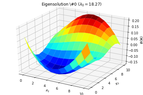 2D_identification_eigensolution_0.png14.3 KB · Views: 239
-
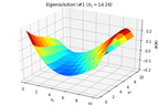 2D_identification_eigensolution_1.png13.4 KB · Views: 258
-
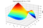 2D_identification_eigensolution_2.png16.3 KB · Views: 235
-
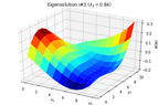 2D_identification_eigensolution_3.png15.8 KB · Views: 235
-
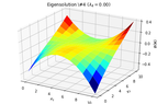 2D_identification_eigensolution_4.png13.9 KB · Views: 257