FEM, Matlab and the modes of an element

[Trying2Learn]

TL;DR Summary

What are the zero-eigenvalue modes of a 4 noded element

Hello

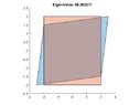
I wrote a Matlab code to form the 8 by 8 stiffness matrix of a single, 4-noded element, for a plane strain problem for an isotropic element.

I conduct an eigenvalue analysis on this matrix

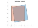
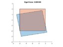
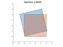
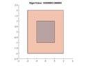
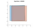
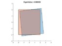
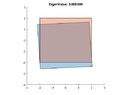
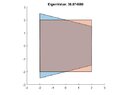
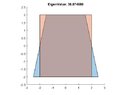
Matlabe reports 5 non-zero eigenvalue modes, and 3 zero-eigenvalue modes (as expected)

Of the 3 zero-eigenvalue vectors, I KNOW that there should be two pure translations (one in each direction) and one rotation.

(I am doing this because I want to see the hourglass modes, out of interest, but i cannot even get that far to under-integrate, yet)

I am doing this in Matlab and I am getting my three zero-eigenvalue "vectors" and they look like this, below (first three images)

I can see that all three manifest free body translation and rotations (some have some deformation, but I can ignore that, for now).

The question is: what can (or should) I do to (in the Matlab code) so that these three zero eigenvalue modes, visualize as two pure translations and one rotation?

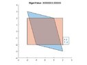
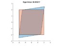
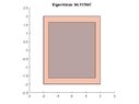
For the hell of it, I also plot TWO of the five non-zero eigenvalue modes (these are all what I expect)

(And to be honest, I would like to remove some of the deformation from the free body modes, too; and the fifth one seems to have pure shear but ALSO a rotation)

It seems as if Matlab is reporting combinations of the eigenvecors (and that makes no sense to me) -- unless I am very confused.

 

[Arjan82]

You can check that $\phi^T M \phi = I$. (if not $I$ then at least a diagonal matrix) If that is true, then the eigenvectors are not a combination of each other.

How do you deal with isoparametricy? (is that a word..? but for quad elements you need an isoparametric formulation)

 

[Arjan82]

Also: make these plots with the

axis equal

command, such that you get the true shapes of the elements

 

[Trying2Learn]

You can check that $\phi^T M \phi = I$. (if not $I$ then at least a diagonal matrix) If that is true, then the eigenvectors are not a combination of each other.

How do you deal with isoparametricy? (is that a word..? but for quad elements you need an isoparametric formulation)

Can I expand on this?

When the eigenvalues are the same, one can add the associated eigenvectors, and still get an eigenvector: not issue there.

Now in a modal analysis of a quad finite element, there are three zero eigenvalues (you see them, above)

I KNOW that they represent: translation in one direction, translation in a second, and a rotation.

I look at those first three modes above and can almost see the two translations and rotaitons, combined.

My question is this... How can I get Matlab to give me those shapes?

Or, another way, how did they first figure it out? It seems they had to have anticipated, in advance, that there are two translations and a rotation. What is happening in Matlab that is not giving me those, but a combination of them.
Should I have to write a code to actually compute the three eigenvectors by first anticipating the form?

 

[Arjan82]

When the eigenvalues are the same, one can add the associated eigenvectors, and still get an eigenvector: not issue there.

True, but if you combine the eigenvectors, they are not orthogonal anymore and thus $\phi^T M \phi = I$ does not hold anymore ($\phi$ the vector with all your DOFs, $M$ the mass matrix, $I$ the identity matrix).

What command do you use? Just the 'eig' command? It should be something like this:

[phi, lamb] = eig(K,M);

With K the stiffness matrix and M the mass matrix.

 

[Arjan82]

True, ...

Actually, not really true. If you combine eigenvectors, they are not eigenvectors anymore... They're supposed to be orthogonal to each other.

 

[Trying2Learn]

True, but if you combine the eigenvectors, they are not orthogonal anymore and thus $\phi^T M \phi = I$ does not hold anymore ($\phi$ the vector with all your DOFs, $M$ the mass matrix, $I$ the identity matrix).

What command do you use? Just the 'eig' command? It should be something like this:

[phi, lamb] = eig(K,M);

With K the stiffness matrix and M the mass matrix.

Yes, I use the Eig, but this is not a dynamics problem, so there is no mass matrix.

I am just evaluating the plane strain stiffness matrix and computing those eigenvalues.

I get them correct (see pictures), but I do not like the form.

I KNOW that the three zero eigenvalue vectors should be two translations and a rotation

But Matlab does not give me those preferred eigenvectors: It gives me combinations of them.

 

[Arjan82]

You are repeating yourself, I understand the question already the first time...

Also, I don't know about an eigenvalue problem in FEM that does not use the mass matrix. What you are computing, normally, are vibration modes and frequency, which is indeed a dynamics problem. I don't know what you would get if you only use K as input (I've never read about that anywhere in any book...). What physics would be behind that?

 

[Trying2Learn]

You are repeating yourself, I understand the question already the first time...

Also, I don't know about an eigenvalue problem in FEM that does not use the mass matrix. What you are computing, normally, are vibration modes and frequency, which is indeed a dynamics problem. I don't know what you would get if you only use K as input (I've never read about that anywhere in any book...). What physics would be behind that?

No, you do NOT need the mass matrix

You take the B matrix that relates strain and displacements and form this as the elemental stiffness matrix
(See image)

That is an 8 by 8 matrix

There will be 3 0-eigenvalue eigenvectors (free body displacement in two directions and one rotation); and five non-zero eigenvalue eigenvectors.

I am beginning to think it is a Matlab issue when the eigenvalues are the same. Eig() reports any legit. eigenvector.

But I am trying to get it to report the vectors in two translations and one rotation form.

As an extension...

For example, if I under-integrate, there are now five zero-eigenvalues (with the two new vectors evincing the hour glass modes): I get these from my code. However, I have the same problem there. Matlab is just reporting back any combination of the displacements and rotations and the two hour glass modes.

 

[Arjan82]

No, you do NOT need the mass matrix

That's not an answer to my question, let me try again: what physics are you trying to solve here? I don't know a physical interpretation of the eigenvectors of only the stiffness matrix.

You take the B matrix that relates strain and displacements and form this as the elemental stiffness matrix
(See image)

That is an 8 by 8 matrix

Ok, what you are showing is a formula which defines the element stiffness matrix (which includes the isoparametric formulation, so thanks for answering that question...). But I really don't know what you are trying to say with that. I know how to get a stiffness matrix.

There will be 3 0-eigenvalue eigenvectors (free body displacement in two directions and one rotation); and five non-zero eigenvalue eigenvectors.

So, again, I know this is true for the dynamical problem, so if you include the mass matrix. I really don't know what you get when you use only the stiffness matrix, of course you CAN solve for eigenvectors using only the stiffness matrix, but I don't know how to interpret the results. How are you so sure you would get this answer? Do you have a reference?

I am beginning to think it is a Matlab issue when the eigenvalues are the same. Eig() reports any legit. eigenvector.

I can assure you: it is NOT Matlab. Matlab is an acronym for Matrix Laboraty, so solving matrix problems is its purpose in life... It is developed over decades and since the eigenvalue problem is one of the most basic problems, it is probably one of the first functions they implemented...

But I am trying to get it to report the vectors in two translations and one rotation form.

That is very clear by now... I'm trying to help you, but you need to help me understand what you are doing as well...

As an extension...

For example, if I under-integrate, there are now five zero-eigenvalues (with the two new vectors evincing the hour glass modes): I get these from my code. However, I have the same problem there. Matlab is just reporting back any combination of the displacements and rotations and the two hour glass modes.

So, the 'eig' command computes the eigenvectors of the matrix you put in (the stiffness matrix in your case). These are by definition orthogonal so NOT any combination of eigenvectors. You can check that yourself by computing $\phi^T K \phi$: if that equals a diagonal matrix, then your set of eigenvectors are orthogonal.

In other words: your problem is really in your own computation, not anywhere else...

 

[Trying2Learn]

That's not an answer to my question, let me try again: what physics are you trying to solve here? I don't know a physical interpretation of the eigenvectors of only the stiffness matrix.
Ok, what you are showing is a formula which defines the element stiffness matrix (which includes the isoparametric formulation, so thanks for answering that question...). But I really don't know what you are trying to say with that. I know how to get a stiffness matrix.
So, again, I know this is true for the dynamical problem, so if you include the mass matrix. I really don't know what you get when you use only the stiffness matrix, of course you CAN solve for eigenvectors using only the stiffness matrix, but I don't know how to interpret the results. How are you so sure you would get this answer? Do you have a reference?
I can assure you: it is NOT Matlab. Matlab is an acronym for Matrix Laboraty, so solving matrix problems is its purpose in life... It is developed over decades and since the eigenvalue problem is one of the most basic problems, it is probably one of the first functions they implemented...
That is very clear by now... I'm trying to help you, but you need to help me understand what you are doing as well...
So, the 'eig' command computes the eigenvectors of the matrix you put in (the stiffness matrix in your case). These are by definition orthogonal so NOT any combination of eigenvectors. You can check that yourself by computing $\phi^T K \phi$: if that equals a diagonal matrix, then your set of eigenvectors are orthogonal.

In other words: your problem is really in your own computation, not anywhere else...

I do not remember the book. But I know that 30 years ago, I actually calculated them.

A few months ago, I asked if it was true, and someone responded
https://www.physicsforums.com/threads/the-8-mode-shapes-of-a-plane-finite-element.1014037/

However now that I had the time, I wrote the code myself and got similar shapes. And I recall, 30 years ago, in some book (I do not remember), that one can interpret the modes of a single element. And this would go a long way to explain why one must apply proper boundary conditions: to stop the free body mode.

I also recall doing it for an under-integration and seeing the additional two hourglass modes. I long since lost the work I did, and I cannot remember where I read it. But I KNOW that the book, back then, interpreted the modes of a single element like this.

 

[Arjan82]

Ok, if I look at the shapes that @FEAnalyst provided using Abaqus, they are also not perfectly in the two translation and single rotation form. The first three shapes there are also somewhat of a combination.

 

[Trying2Learn]

Yes and that is exactly my point. Three of those shapes are three zero-eigen value vectors.

And I KNOW the book, 30 years ago, said that they represent 2 translations and one rotation.

And I know that a repeated eigenvalue (in this case, zero) has eigen vectors that can be added and produce another eigenvector.

So I have a core belief that there must be a way to alter those first three eigenvectors from Matlab, to these three

(Numbering the nodes CCW from bottom left, with x-displacement followed by y)
1 0 1 0 1 0 1 0
0 1 0 1 0 1 0 1
1 -1 1 1 -1 1 -1 -1

Naturally, I would normalize themSee, I think it is a Matlab (not problem, but Issue). It reports back the fist three modes, but I KNOW that I once saw this as the three above

 

[Trying2Learn]

Ok, if I look at the shapes that @FEAnalyst provided using Abaqus, they are also not perfectly in the two translation and single rotation form. The first three shapes there are also somewhat of a combination.

BTW: one more issue, to note

I created those mode shapes using the modulus of steel and some Poisson ratio.
If I use a much lower modulus (by several magnitudes), then Matlab starts reporting back three modes that START to look like ONLY translation in x, ONLY translation in y, and ONLY rotation (but they still all have aspects of each other)

 

[Arjan82]

So, in that case you are asking the question how to scale and sum all eigenvectors to get [1 0 1 0 ...] right?

But that's an easy problem to solve (I assumed that you have your stiffness matrix K already defined):

f = [1 0 1 0 1 0 1 0]';

[phi, lamb] = eig(K);

phi_inv = phi^(-1);
s = phi_inv*f;

# Now check:
f2 = phi*s

#f and f2 should be equal

So, now you have a set of scale factors in the vector 's' that scales your eigenvectors such that the combination of eigenvectors results in f = [1 0 1 0 1 0 1 0]'.

If you are right, then 's' should only have non-zero values in the first three elements.

 

[Trying2Learn]

So, in that case you are asking the question how to scale and sum all eigenvectors to get [1 0 1 0 ...] right?

But that's an easy problem to solve (I assumed that you have your stiffness matrix K already defined):

f = [1 0 1 0 1 0 1 0]';

[phi, lamb] = eig(K);

phi_inv = phi^(-1);
s = phi_inv*f;

# Now check:
f2 = phi*s

#f and f2 should be equal

So, now you have a set of scale factors in the vector 's' that scales your eigenvectors such that the combination of eigenvectors results in f = [1 0 1 0 1 0 1 0]'.

If you are right, then 's' should only have non-zero values in the first three elements.

OK, I will do that tomorrow. I believe it will work. But my question remains: how can I get eig() to send back eigenvectors where *I* have some input into how it handles vectors from repeated eigenvalues?

I KNOW I did this with IMSL years ago.

 

[Trying2Learn]

So, in that case you are asking the question how to scale and sum all eigenvectors to get [1 0 1 0 ...] right?

But that's an easy problem to solve (I assumed that you have your stiffness matrix K already defined):

f = [1 0 1 0 1 0 1 0]';

[phi, lamb] = eig(K);

phi_inv = phi^(-1);
s = phi_inv*f;

# Now check:
f2 = phi*s

#f and f2 should be equal

So, now you have a set of scale factors in the vector 's' that scales your eigenvectors such that the combination of eigenvectors results in f = [1 0 1 0 1 0 1 0]'.

If you are right, then 's' should only have non-zero values in the first three elements.

Or this...

You showed me how to verify that the 1 0 1 0 1 0 1 0 is an eigenvector...
But how would I have known that to begin with?
How can I recombine the zero-eigenvalue eigenvectors from Matlab, to produce the pure displacements and the rotations?

 

[Arjan82]

You showed me how to verify that the 1 0 1 0 1 0 1 0 is an eigenvector...

Nope... the 10101010 vector is NOT an eigenvector... It is a linear combination of eigenvectors. So what is the defining property of an eigenvector:

if $\phi$ is an eigenvector of matrix $K$, and $\lambda$ its eigenvalue, then it must hold that:

$$K \phi - \lambda \phi = 0$$

Now a bit of MATLAB code to show that this does not work for the 01010101 vector:

% Some random 8x8 matrix, as long as it is not singular it is ok:
K = reshape((1:64),8,8);

% Indices of the diagonal:
n = (1:9:64)';

% Make the diagonal larger such that the eigenvalues are all positive and
% real:
K(n) = K(n)*10;

% Compute eigenvectors:
[phi, lamb] = eig(K);

% Define the 0101010101 matrix in a lazy way:
f = repmat([1; 0], 4,1);

% Now check that (K-lambda * I)phi = 0. This means that K*phi is equal to
% phi but scaled. So we divide element by element with phi and make sure
% that all values in the vector are equal (and in fact equal to lambda).
% So, for the first eigenvector:
>> K*phi(:,1)./(phi(:,1))

ans =

  734.1328
  734.1328
  734.1328
  734.1328
  734.1328
  734.1328
  734.1328
  734.1328% The second vector:
>> K*phi(:,2)./(phi(:,2))

ans =

    8.0116
    8.0116
    8.0116
    8.0116
    8.0116
    8.0116
    8.0116
    8.0116

% This all checks out, but now with the vector f:
>> K*f./f

ans =

   109
   Inf
   279
   Inf
   449
   Inf
   619
   Inf

% And this does not work... Also, note the infinities, this meains that f
% is simply never going to be an eigenvector of K...

But how would I have known that to begin with?
How can I recombine the zero-eigenvalue eigenvectors from Matlab, to produce the pure displacements and the rotations?

So, I've above shown you how to compute the vector s. That is literally what you are asking for. It is a vector that together with the matrix of eigenvectors combines to produce the pure displacement... So s is a list of scaling factors by which to scale all eigenvectors, and if you then add them all up, they become the pure displacement vector in x.

So, if only the eigenvectors belonging to the zero-eigenvalues can be combined to produce pure displacements, that means that the values of s belonging to the zero-eigenvectors should be non-zero. The other values in s should then be zero. Please check and let me know if that is true.

 

[Trying2Learn]

I am still not convinced.

If you wish, I can send you the entire Matlab code. But, for now, it produces the following stiffness matrix for a plane strain problem. YOUR code, above, used a random matrix.

Here are the material properties I used in the 3 by 3 D matrix
E = 20.;
nu = 0.15;
D = (E/(1-nu)/(1+nu)) * [1, nu, 0; nu, 1, 0; 0, 0, 0.5*(1-nu)];

When I do 2 point Gauss itegration in each direction, I get this as the stiffness matrix

K =

38.8747 11.7647 -21.4834 -5.6266 -19.4373 -11.7647 2.0460 5.6266
11.7647 38.8747 5.6266 2.0460 -11.7647 -19.4373 -5.6266 -21.4834
-21.4834 5.6266 38.8747 -11.7647 2.0460 -5.6266 -19.4373 11.7647
-5.6266 2.0460 -11.7647 38.8747 5.6266 -21.4834 11.7647 -19.4373
-19.4373 -11.7647 2.0460 5.6266 38.8747 11.7647 -21.4834 -5.6266
-11.7647 -19.4373 -5.6266 -21.4834 11.7647 38.8747 5.6266 2.0460
2.0460 -5.6266 -19.4373 11.7647 -21.4834 5.6266 38.8747 -11.7647
5.6266 -21.4834 11.7647 -19.4373 -5.6266 2.0460 -11.7647 38.8747

If you work with this matrix (you do not need to see how I got it, but I would be happy to post the entire code), you will get the eigenvalues and eigenvectors similar to the top of this thread (the ones a the top used a much higher Young Mod. However the, this current matrix has a MUCH lower Youngs' Modulus, and the eigenvectore here, REALLY LOOK like the first three are a pure translation, pure translatoin and pure rotation (with elements of each, combined)

If, however, I multiply the K, above, by any of these three, below (translation in x, in y, and rotation), I get the zero vector (informing me that each of these three is an eigenvector because they produce a zero vector when multiplied by K:

K * Mode 1 = Lamba * Mode 1 (where Lambda is the zero eigenvalue)Mode1 = [1;0;1;0;1;0;1;0]
Mode2 = [0;1;0;1;0;1;0;1]
Mode3 = [1;-1;1;1;-1;1;-1;-1]

In fact, I will post the results from Matlab. Unlike the ones above, these have a much lower Young modulus and notice that Matlab is BEGINNING to report the zero eigenvalue modes as pure translations and a rotation.

It seems to me that eig (From Matlab) is producing all correct eigenvalues and vectors, but I just do not like the eigenvectors it produces when the eigenvalues are repeated. I much prefer to somehow see two PURE translations and one rotaiotn.

 

[Trying2Learn]

IN fact, here is the Matlab code in its entirety

function FourPointCounterCW()

clear
clc
close all

% Establish the material properties
E = 20.;
nu = 0.15;
D = (E/(1-nu)/(1+nu)) * [1, nu, 0; nu, 1, 0; 0, 0, 0.5*(1-nu)];

% Assert the gauss point
g = 1/sqrt(3);

% Assert the global nodes (just for fun to check the determinant of the Jacobian)
X1 = -2;
Y1 = -2;

X2 = 2;
Y2 = -2;

X3 = 2;
Y3 = 2;

X4 = -2;
Y4 = 2;%These are crudely written functions, that could be written better, but
%they are fine% GAUSS POINT 1
r = -g;
s = -g;
%This function evaluates the B and Stiffnes matrix at the gauss point
B1 = getB(r,s);
dJ1 = getdJ(r, s, X1, Y1, X2, Y2, X3, Y3, X4, Y4);
K1 = B1'*D*B1*dJ1;
% GAUSS POINT 2
r = +g;
s = -g;
%This function evaluates the B and Stiffnes matrix at the gauss point
B2 = getB(r,s);
dJ2 = getdJ(r, s, X1, Y1, X2, Y2, X3, Y3, X4, Y4);
K2 = B2'*D*B2*dJ2;

% GAUSS POINT 3
r = +g;
s = +g;
%This function evaluates the B and Stiffnes matrix at the gauss point
B3 = getB(r,s);
dJ3 = getdJ(r, s, X1, Y1, X2, Y2, X3, Y3, X4, Y4);
K3 = B3'*D*B3*dJ3;% GAUSS POINT 4
r = -g;
s = +g;
B4 = getB(r,s);
dJ4 = getdJ(r, s, X1, Y1, X2, Y2, X3, Y3, X4, Y4);
K4 = B4'*D*B4*dJ4;%Add the four values. This means we are doing the integration
%to get the stiffness
K = K1 + K2 + K3 + K4;
J = dJ1 + dJ2 + dJ3 + dJ4

%Get the eigenvalues and mode shapes
[V,D] = eig(K, 'vector', 'nobalance');%these two lines reorder the eigevalues and eigenvectors so lowest is first
[D, ind] = sort(D);
V = V(:, ind)
% Plot the mode shapes
for i = 1:8

% Remember you must ADD to the displacement, the original location of the
% node

X1p = X1 + V(1,i);
Y1p = Y1 + V(2,i);

X2p = X2 + V(3,i);
Y2p = Y2 + V(4,i);

X3p = X3 + V(5,i);
Y3p = Y3 + V(6,i);

X4p = X4 + V(7,i);
Y4p = Y4 + V(8,i);

figure(i)
hold on
title(sprintf('EigenValue: %f', D(i)));
pgon = polyshape([X1p X2p X3p X4p],[Y1p Y2p Y3p Y4p]);
pgon0 = polyshape([X1, X2, X3, X4],[Y1, Y2, Y3, Y4]);
plot(pgon);
plot(pgon0);
pbaspect([1 1 1])
hold offend

%%this is a test to see if I get the null vector when the stiffness
%%matrix multiplies what I believe to be three eigenvectors

Mode1 = [1;0;1;0;1;0;1;0]
Mode2 = [0;1;0;1;0;1;0;1]
Mode3 = [1;-1;1;1;-1;1;-1;-1]

K*Mode1
K*Mode2
K*Mode3
endfunction B = getB(r, s)

%This function will need the values of the derviatives of the shape
%functions, CARTESIONALLY, which is the same as LOCALLY

%Notation: N1r is partial N1/ Partial r
% the f is the function, down bleow.

%Now look at page 9
%x varies as r
%x does not vary with s (remember we aligned the element to match the idealN1r = fN1r(r,s);
N2r = fN2r(r,s);
N3r = fN3r(r,s);
N4r = fN4r(r,s);
N1s = fN1s(r,s);
N2s = fN2s(r,s);
N3s = fN3s(r,s);
N4s = fN4s(r,s);

%Now create B: found in the code as the function: quadB

B = [N1r, 0, N2r, 0, N3r, 0, N4r, 0;
0, N1s, 0, N2s, 0, N3s, 0, N4s;
N1s, N1r, N2s, N2r, N3s, N3r, N4s, N4r];

end
%For these functions, open qdkasmbl1.c and look at page 6

function N1r = fN1r(r, s)
N1r = -0.25 * (1-s);
end
function N2r = fN2r(r, s)
N2r = +0.25 * (1-s);
end
function N3r = fN3r(r, s)
N3r = +0.25 * (1+s);
end
function N4r = fN4r(r, s)
N4r = -0.25 * (1+s);
endfunction N1s = fN1s(r, s)
N1s = -0.25 * (1-r);
end
function N2s = fN2s(r, s)
N2s = -0.25 * (1+r);
end
function N3s = fN3s(r, s)
N3s = +0.25 * (1+r);
end
function N4s = fN4s(r, s)
N4s = +0.25 * (1-r);
end

function dJ = getdJ(r, s, X1, Y1, X2, Y2, X3, Y3, X4, Y4)

% remember, global x/y matches to local r/s, so the COLORED terms
%(red, blue, green and pink) are 1 or 0, while the global cartesian are 1
%or -1 in the J matrix on page 10

J(1,1) = fN1r(r,s)*X1 + fN2r(r,s)*X2 + fN3r(r,s)*X3 + fN4r(r,s)*X4;
J(1,2) = fN1r(r,s)*Y2 + fN2r(r,s)*Y2 + fN3r(r,s)*Y3 + fN4r(r,s)*Y4;
J(2,1) = fN1s(r,s)*X1 + fN2s(r,s)*X2 + fN3s(r,s)*X3 + fN4s(r,s)*X4;
J(2,2) = fN1s(r,s)*Y1 + fN2s(r,s)*Y2 + fN3s(r,s)*Y3 + fN4s(r,s)*Y4;

%print J: the off diagonals better be 0 since there is no distortion of global from local (just an expansion)

dJ = J(1,1)*J(2,2) - J(1,2)*J(2,1);

end

 

[Arjan82]

IN fact, here is the Matlab code in its entirety

I also need the functions fNlr, fN2r fN3r fN4r

 

[Trying2Learn]

I also need the functions fNlr, fN2r fN3r fN4r

I think they are all there. The Matlab file contained all the functions, but I did not reformat when I pasted it in.

They are near the bottom.

THANK YOU; by the way.

 

[Trying2Learn]

IN fact, here is the Matlab code in its entirety

function FourPointCounterCW()

clear
clc
close all

% Establish the material properties
E = 20.;
nu = 0.15;
D = (E/(1-nu)/(1+nu)) * [1, nu, 0; nu, 1, 0; 0, 0, 0.5*(1-nu)];

% Assert the gauss point
g = 1/sqrt(3);

% Assert the global nodes (just for fun to check the determinant of the Jacobian)
X1 = -2;
Y1 = -2;

X2 = 2;
Y2 = -2;

X3 = 2;
Y3 = 2;

X4 = -2;
Y4 = 2;%These are crudely written functions, that could be written better, but
%they are fine% GAUSS POINT 1
r = -g;
s = -g;
%This function evaluates the B and Stiffnes matrix at the gauss point
B1 = getB(r,s);
dJ1 = getdJ(r, s, X1, Y1, X2, Y2, X3, Y3, X4, Y4);
K1 = B1'*D*B1*dJ1;
% GAUSS POINT 2
r = +g;
s = -g;
%This function evaluates the B and Stiffnes matrix at the gauss point
B2 = getB(r,s);
dJ2 = getdJ(r, s, X1, Y1, X2, Y2, X3, Y3, X4, Y4);
K2 = B2'*D*B2*dJ2;

% GAUSS POINT 3
r = +g;
s = +g;
%This function evaluates the B and Stiffnes matrix at the gauss point
B3 = getB(r,s);
dJ3 = getdJ(r, s, X1, Y1, X2, Y2, X3, Y3, X4, Y4);
K3 = B3'*D*B3*dJ3;% GAUSS POINT 4
r = -g;
s = +g;
B4 = getB(r,s);
dJ4 = getdJ(r, s, X1, Y1, X2, Y2, X3, Y3, X4, Y4);
K4 = B4'*D*B4*dJ4;%Add the four values. This means we are doing the integration
%to get the stiffness
K = K1 + K2 + K3 + K4;
J = dJ1 + dJ2 + dJ3 + dJ4

%Get the eigenvalues and mode shapes
[V,D] = eig(K, 'vector', 'nobalance');%these two lines reorder the eigevalues and eigenvectors so lowest is first
[D, ind] = sort(D);
V = V(:, ind)
% Plot the mode shapes
for i = 1:8

% Remember you must ADD to the displacement, the original location of the
% node

X1p = X1 + V(1,i);
Y1p = Y1 + V(2,i);

X2p = X2 + V(3,i);
Y2p = Y2 + V(4,i);

X3p = X3 + V(5,i);
Y3p = Y3 + V(6,i);

X4p = X4 + V(7,i);
Y4p = Y4 + V(8,i);

figure(i)
hold on
title(sprintf('EigenValue: %f', D(i)));
pgon = polyshape([X1p X2p X3p X4p],[Y1p Y2p Y3p Y4p]);
pgon0 = polyshape([X1, X2, X3, X4],[Y1, Y2, Y3, Y4]);
plot(pgon);
plot(pgon0);
pbaspect([1 1 1])
hold offend

%%this is a test to see if I get the null vector when the stiffness
%%matrix multiplies what I believe to be three eigenvectors

Mode1 = [1;0;1;0;1;0;1;0]
Mode2 = [0;1;0;1;0;1;0;1]
Mode3 = [1;-1;1;1;-1;1;-1;-1]

K*Mode1
K*Mode2
K*Mode3
endfunction B = getB(r, s)

%This function will need the values of the derviatives of the shape
%functions, CARTESIONALLY, which is the same as LOCALLY

%Notation: N1r is partial N1/ Partial r
% the f is the function, down bleow.

%Now look at page 9
%x varies as r
%x does not vary with s (remember we aligned the element to match the idealN1r = fN1r(r,s);
N2r = fN2r(r,s);
N3r = fN3r(r,s);
N4r = fN4r(r,s);
N1s = fN1s(r,s);
N2s = fN2s(r,s);
N3s = fN3s(r,s);
N4s = fN4s(r,s);

%Now create B: found in the code as the function: quadB

B = [N1r, 0, N2r, 0, N3r, 0, N4r, 0;
0, N1s, 0, N2s, 0, N3s, 0, N4s;
N1s, N1r, N2s, N2r, N3s, N3r, N4s, N4r];

end
%For these functions, open qdkasmbl1.c and look at page 6

function N1r = fN1r(r, s)
N1r = -0.25 * (1-s);
end
function N2r = fN2r(r, s)
N2r = +0.25 * (1-s);
end
function N3r = fN3r(r, s)
N3r = +0.25 * (1+s);
end
function N4r = fN4r(r, s)
N4r = -0.25 * (1+s);
endfunction N1s = fN1s(r, s)
N1s = -0.25 * (1-r);
end
function N2s = fN2s(r, s)
N2s = -0.25 * (1+r);
end
function N3s = fN3s(r, s)
N3s = +0.25 * (1+r);
end
function N4s = fN4s(r, s)
N4s = +0.25 * (1-r);
end

function dJ = getdJ(r, s, X1, Y1, X2, Y2, X3, Y3, X4, Y4)

% remember, global x/y matches to local r/s, so the COLORED terms
%(red, blue, green and pink) are 1 or 0, while the global cartesian are 1
%or -1 in the J matrix on page 10

J(1,1) = fN1r(r,s)*X1 + fN2r(r,s)*X2 + fN3r(r,s)*X3 + fN4r(r,s)*X4;
J(1,2) = fN1r(r,s)*Y2 + fN2r(r,s)*Y2 + fN3r(r,s)*Y3 + fN4r(r,s)*Y4;
J(2,1) = fN1s(r,s)*X1 + fN2s(r,s)*X2 + fN3s(r,s)*X3 + fN4s(r,s)*X4;
J(2,2) = fN1s(r,s)*Y1 + fN2s(r,s)*Y2 + fN3s(r,s)*Y3 + fN4s(r,s)*Y4;

%print J: the off diagonals better be 0 since there is no distortion of global from local (just an expansion)

dJ = J(1,1)*J(2,2) - J(1,2)*J(2,1);

end

And ignore some of the comments. I initially wrote it so that the detJ woud be 1 (and the local and global were the same)

 

[Arjan82]

Ah, I overlooked them indeed.

If I write this at the end of FourPointCounterCW:

Vi = V^-1;

s1 = Vi*Mode1
s2 = Vi*Mode2
s3 = Vi*Mode3

Then I get:

>> s1

s1 =

   0.396662544532026
  -1.660972854131425
  -0.420967911592968
  -0.000000000000000
   0.000000000000001
                   0
  -0.000000000000000
  -0.000000000000000

>> s2

s2 =

   0.925895125244109
   1.077632183627960
  -1.866168969125933
   0.000000000000000
  -0.000000000000000
   0.000000000000000
  -0.000000000000000
  -0.000000000000000

>> s3

s3 =

   4.105654396502303
   3.321945708262850
   0.841935823185934
  -0.000000000000000
   0.000000000000000
  -0.000000000000001
  -0.000000000000000
  -0.000000000000000

You see that in all cases s is only nonzero for the first 3 values (ignoring numerical noise). Since the first 3 values of D are also zero, this means these are the vectors for pure translation and rotation. So now you can combine only the first 3 eigenvectors (which are for the pure translations and rotations):

>> V(:,1:3) * s1(1:3)

ans =

   1.000000000000000
   0.000000000000000
   0.999999999999999
   0.000000000000000
   1.000000000000000
  -0.000000000000000
   1.000000000000000
   0.000000000000000
  
>> V(:,1:3) * s2(1:3)

ans =

   0.000000000000000
   1.000000000000000
                   0
   1.000000000000000
  -0.000000000000000
   1.000000000000000
   0.000000000000000
   1.000000000000000

>> V(:,1:3) * s3(1:3)

ans =

   1.000000000000000
  -1.000000000000000
   0.999999999999999
   1.000000000000000
  -1.000000000000000
   1.000000000000000
  -0.999999999999999
  -1.000000000000000

And you get back your vectors Mode1, Mode2 and Mode3.

 

[Trying2Learn]

Quick question... why are you testing it by multiplying by the inverse of the stiffness?

I test by multiplying by the stiffness.

 

[Trying2Learn]

And even then, yes, I can see I recapture those modes.

But my core question has always been: why does Matlab report the first three zero-eigenvalue modes as combinations of "what I believe to be pure translations and rotation" I know the e.vectors FROM MATLAB are fine. I just don't like the way they look. That is what I am getting at.

 

[Arjan82]

No, I test with the original V, this is the test:

>> V(:,1:3) * s1(1:3)

because it gives back the original Mode1 vector which I used to compute s1.

I compute s1 with the inverse of the stiffness:

Vi = V^-1;

s1 = Vi*Mode1
s2 = Vi*Mode2
s3 = Vi*Mode3

So now you have the vectors s1 to s3 which contain the scaling values. You can use s1 to s3 to scale the first 3 eigenvectors (V(:,1:3)) to get back Mode1 to Mode3. In other words: you can use s1 to s3 to combine the eigenvectors for the zero value eigenvalues to get pure translation and rotation.

 

[Trying2Learn]

No, I test with the original V, this is the test:

>> V(:,1:3) * s1(1:3)

because it gives back the original Mode1 vector which I used to compute s1.

I compute s1 with the inverse of the stiffness:

Vi = V^-1;

s1 = Vi*Mode1
s2 = Vi*Mode2
s3 = Vi*Mode3

So now you have the vectors s1 to s3 which contain the scaling values. You can use s1 to s3 to scale the first 3 eigenvectors (V(:,1:3)) to get back Mode1 to Mode3. In other words: you can use s1 to s3 to combine the eigenvectors for the zero value eigenvalues to get pure translation and rotation.

OK, I understand and I like that.

But now the closing question

Matlab reports these eigenvectors and I do not like the way they look. If I am a first time FE coder and I experiment to see the modes, and get those shapes, NOTHING in them informs me that three of the eigenvectors would have been MORE INFORMATIVE had I seen them as pure translations and one pure rotation. How would I have known this in advance. In other words: the eigenvectors from Matlab (sorry, there is no other way to say this) "displease" me (they are not pretty). The author of that book (from 30 years ago, I forgot the name), somehow KNEW this to be true (is that simply the mark of an intuitive engineer)? Did s/he get lucky getting pure eigenvectors, when s/he coded it for his/her book?

 

[Arjan82]

And even then, yes, I can see I recapture those modes.

Good, because that was literally your question:

How can I recombine the zero-eigenvalue eigenvectors from Matlab, to produce the pure displacements and the rotations?

But my core question has always been: why does Matlab report the first three zero-eigenvalue modes as combinations of "what I believe to be pure translations and rotation"

Because K is singular, so the eigenvalues are 0. This means that any any combination of the eigenvectors belonging to the 0 eigenvalues is also an eigenvector, this is not generally the case as I've shown before!

This being the case the algoritm in 'eig' needs to choose 'some' eigenvectors. Since the programmers didn't bother to make sure the end result was 'beautiful' it just comes up with some combination of eigenvectors which are valid.

I know the e.vectors FROM MATLAB are fine. I just don't like the way they look. That is what I am getting at.

Beauty is in the eye of the beholder... I think MathWorks thinks the result is absolutely pulchritudinous... But most importantly, they are correct...

 

[Trying2Learn]

Good, because that was literally your question:
Because K is singular, so the eigenvalues are 0. This means that any any combination of the eigenvectors belonging to the 0 eigenvalues is also an eigenvector, this is not generally the case as I've shown before!

This being the case the algoritm in 'eig' needs to choose 'some' eigenvectors. Since the programmers didn't bother to make sure the end result was 'beautiful' it just comes up with some combination of eigenvectors which are valid.Beauty is in the eye of the beholder... I think MathWorks thinks the result is absolutely pulchritudinous... But most importantly, they are correct...

THANK YOU.

Thanks for the comment, too, on what Matlab considers beautiful. That was my issue. I suppose the person who wrote the book, years ago, just knew it, and used an IMSL routine (and I used one), that just happened to spit them out in a way "I liked."

But I am happy with this, now

Thank you, again.

 

[Arjan82]

Matlab reports these eigenvectors and I do not like the way they look. If I am a first time FE coder and I experiment to see the modes, and get those shapes, NOTHING in them informs me that three of the eigenvectors would have been MORE INFORMATIVE had I seen them as pure translations and one pure rotation. How would I have known this in advance.

Well, the zero-valued eigenvalues is a big give-away... They never occur for fully constraint problems.

 

[Trying2Learn]

Well, the zero-valued eigenvalues is a big give-away... They never occur for fully constraint problems.

And, oddly, THAT was what I wanted to hear. Those last two sentences, were what I was looking for. And, now that you said them, it is obvious. I should have known that.

Thank you for patience (I know I can be stubborn -- sorry if it came across that way).

 

[Arjan82]

Well, we took some detour, but we got there in the end :) All is ok!