PeteyCoco
- 37
- 1
The Function To Be Programmed
[itex]\sigma_m=\frac{4(n_r^2 -1)J_m(n_r k R)}{\pi^2kD_m^+(kR)D_m^-(kR)}[/itex]
where
[itex]D_m(z)=n_rJ'_m(n_rz)H_m(z)-J_m(n_rz)H'_m(z)[/itex].
The '+'/'-' superscripts indicate the limits as z approaches the branch cut, which lies along the negative imaginary half axis, from the positive and negative real sides. The J's and H's are the Bessel functions and Hankel functions of the first kind. I wish to plot this function along the negative imaginary half-axis with respect to k.
My Code
I'm coding this in Python using NumPy and SciPy. Here is my code at present:
With the help of others, I have successfully moved the cut of the Hankel and Neumann functions from the negative real axis to the negative imaginary axis using argument transforms found here. You can confirm this by running the program and plotting the _imcut functions versus their regular counterparts.
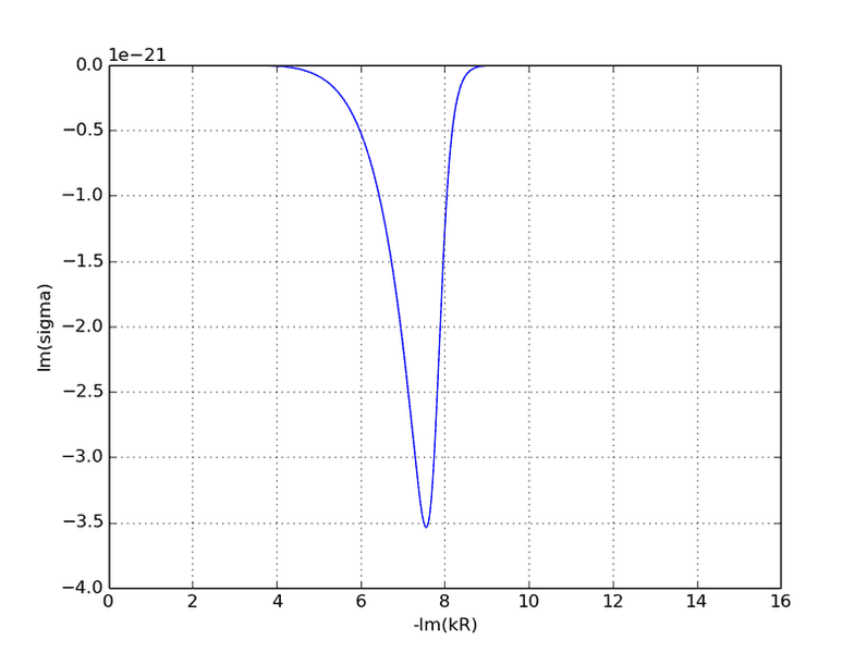
Here's the plot of sigma.imag along the negative imaginary semi-axis:

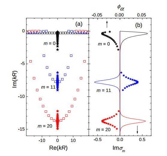
Here's what it should look like (look at the blue m=11 curve at right):

As you can see, it looks sort of right, but it's taking on the wrong values.
These equations and the graph come from page 4 in this article: http://arxiv.org/pdf/1302.0245v1.pdf. Something that the article mentions is that sigma should be a purely imaginary function. I examined the function to see what could be making it part real and part imaginary in my case. I found that the Dm's in the denominator of sigma have equal real and opposite imaginary parts, so I expanded the product to ensure that it comes out purely real (the precision of the two numbers lead to an imaginary part which shouldn't have been there). Still, it isn't working out. Any help would be appreciated! I've been stumped for half of the summer by this one.
[itex]\sigma_m=\frac{4(n_r^2 -1)J_m(n_r k R)}{\pi^2kD_m^+(kR)D_m^-(kR)}[/itex]
where
[itex]D_m(z)=n_rJ'_m(n_rz)H_m(z)-J_m(n_rz)H'_m(z)[/itex].
The '+'/'-' superscripts indicate the limits as z approaches the branch cut, which lies along the negative imaginary half axis, from the positive and negative real sides. The J's and H's are the Bessel functions and Hankel functions of the first kind. I wish to plot this function along the negative imaginary half-axis with respect to k.
My Code
I'm coding this in Python using NumPy and SciPy. Here is my code at present:
import scipy as sp
import numpy as np
import matplotlib.pyplot as plt
from numpy import pi
from scipy.special import jv, iv, kv, jvp, ivp, kvp
m = 11 # Mode number
nr = 2 # Index of refraction
R = 1 # Radius of cylinder
eps = 10e-8 # The Dm's in the denominator are evaluated an amount eps to the left and right of the cutdef yv_imcut(n, z):
return -2/(pi*(1j)**n)*kv(n, -1j*z) + 2*(1j)**n/pi * (0.5j*pi) * iv(n,-1j*z)
def yvp_imcut(n, z):
return (n/z)*yv_imcut(n,z) - yv_imcut(n+1,z)
def hankel1_imcut(n, z):
return jv(n, z) + 1j*yv_imcut(n, z)
def h1vp_imcut(n, z):
return jvp(n, z, 1) + 1j*yvp_imcut(n, z)
# Define the characteristic equation
def Dm(n, z):
return nr*jvp(n, nr*z, 1) * hankel1_imcut(n, z) - jv(n, nr*z)*h1vp_imcut(n,z)
# Define the cut pole density function. The product in the denominator has been written out explicitly for computational reasons.
def sigma(k,n):
return 4*(nr**2 - 1)*jv(n,nr*k*R)/(pi**2 * k * ((Dm(n, k*R-eps).real)**2 + (Dm(n, k*R+eps).imag)**2))
k = np.linspace(0, -15j,1000)
y = sigma(k,m)
x = np.linspace(0,15,1000)
plt.plot(x, y.imag)
plt.show()
With the help of others, I have successfully moved the cut of the Hankel and Neumann functions from the negative real axis to the negative imaginary axis using argument transforms found here. You can confirm this by running the program and plotting the _imcut functions versus their regular counterparts.
Here's the plot of sigma.imag along the negative imaginary semi-axis:
Here's what it should look like (look at the blue m=11 curve at right):
As you can see, it looks sort of right, but it's taking on the wrong values.
These equations and the graph come from page 4 in this article: http://arxiv.org/pdf/1302.0245v1.pdf. Something that the article mentions is that sigma should be a purely imaginary function. I examined the function to see what could be making it part real and part imaginary in my case. I found that the Dm's in the denominator of sigma have equal real and opposite imaginary parts, so I expanded the product to ensure that it comes out purely real (the precision of the two numbers lead to an imaginary part which shouldn't have been there). Still, it isn't working out. Any help would be appreciated! I've been stumped for half of the summer by this one.
Last edited: