Time Series: stationary AR(1) -> MA(infinity)

Click For Summary
SUMMARY

A stationary AR(1) model can be expressed as an MA(infinity) process. The confusion arises when transitioning from the second last line to the final line of the proof, particularly regarding the term Yt-m. As m approaches infinity, φ^m approaches 0, but the behavior of Yt-m must also be considered. The key conclusion is that if Yt is a stationary random variable and |φ| < 1, then the limit of φ^m Yt-m approaches 0 almost surely.

PREREQUISITES
  • Understanding of stationary AR(1) models
  • Knowledge of MA(infinity) processes
  • Familiarity with limits in probability theory
  • Concept of random variables and their behavior
NEXT STEPS
  • Study the properties of stationary processes in time series analysis
  • Learn about the relationship between AR and MA models in time series
  • Explore the concept of almost sure convergence in probability theory
  • Investigate the implications of random variables in limit theorems
USEFUL FOR

Statisticians, data scientists, and anyone involved in time series analysis, particularly those working with AR and MA models.

kingwinner
Messages
1,266
Reaction score
0
Theorem:
A stationary AR(1) model can be expressed in terms of MA(infinity).

Proof:
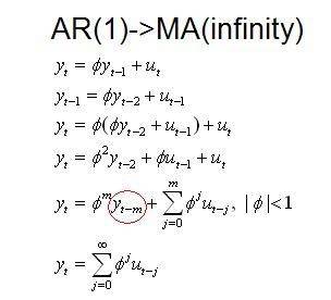
stat5.JPG


Now I don't understand how they get from the second last line to the last line. Where did the term Yt-m go?

I understand you can keep doing the substitution iteratively, but you always have to end up with a "Y" term no matter how many times you do it, but on the last line of the proof there is no "Y" term, so it magically disappared? I'm really confused.

Hopefully someone can explain this (in simple terms if possible). Thank you!
 
Physics news on Phys.org
They're taking the limit as \phi goes to infinity. What happens to \phi^m in that limit?
 
I think it's the limit as m->∞.

As m->∞,
φm ->0
BUT you also have to look at what happens to the other term, right? What if Yt-m->∞? Then we have indeterminate form 0*∞, and we just can't conclude that the product->0.
(Also, another complication is that Yt-m is a random variable, so I'm not sure if all of these make sense or not.)
 
kingwinner said:
I think it's the limit as m->∞.
You're right -- sorry.

As m->∞,
φm ->0
BUT you also have to look at what happens to the other term, right? What if Yt-m->∞? Then we have indeterminate form 0*∞, and we just can't conclude that the product->0.

(Also, another complication is that Yt-m is a random variable, so I'm not sure if all of these make sense or not.)
I'll take those two complications in reverse order. First, the equation will in general be true "almost surely", meaning with probability 1. It may be possible for \phi^m y_{t-m} to approach a constant or diverge, but this happens with probability 0. Second, you have to know SOMETHING about the y's. If this is the same book that your random walk problem came from, maybe they left out essential information. But the key fact is there in the word "stationary". It takes a little work to prove it, but If y is a decently-behaved RV (i.e., has a CDF) and is stationary and |\phi|&lt;1, then \lim_{m\to\infty}\phi^m y_{t-m}=0 almost surely.
 

Similar threads

  • · Replies 10 ·
Replies
10
Views
3K
  • · Replies 14 ·
Replies
14
Views
3K
  • · Replies 1 ·
Replies
1
Views
1K
  • · Replies 1 ·
Replies
1
Views
1K
  • · Replies 7 ·
Replies
7
Views
5K
  • · Replies 3 ·
Replies
3
Views
2K
  • · Replies 3 ·
Replies
3
Views
5K
  • · Replies 2 ·
Replies
2
Views
3K
  • · Replies 3 ·
Replies
3
Views
2K
  • · Replies 10 ·
Replies
10
Views
3K