MATLAB Turning Fourier coefficients into an interpolated freq domain function

[skynelson]

TL;DR

Using Fourier series to generate a smooth function, then using Fourier transform to generate a smooth curve of the original coefficient distribution.

Hi, I am interested in understanding the relationships between Fourier series and Fourier transform better. My goal is
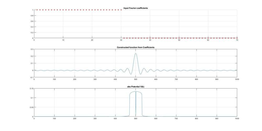
1) Start with a set of ordered numbers representing Fourier coefficients. I chose to create 70 coefficients and set the first 30 to the value 1 and the remaining to zero.
2) Take those coefficients as the amplitudes of plane waves, whose frequency corresponds to the index of the coefficient in the ordered list. Add all these waves together to get a smooth curve (a sinc function).
3) Use the native function fft to try to generate a continuous rect function, corresponding to the sinc function.

This final curve would be the continuous version of the original coefficients, as if they were interpolated.
The first two steps seem successful, but the reproduced rect function is curved on the corners. I suspect this may have something to do with not handling the imaginary portion properly.

Any help getting the code to do what I want would be appreciated! (And any additional wisdom on the goal of this endeavor relating the Fourier series and Fourier transform and interpolation of the Fourier coefficients would be welcome too! Is it a fool's errand?) [CODE lang="matlab" title="MATLAB Code" highlight="24,33,38"]domain = 1000;
PotentialSize = 70;
X = linspace(1,70,70);
Vbk = zeros(1, PotentialSize);
Vbk(1:30) = 1;

%% PLOT FIGURE
figure('units','normalized','outerposition',[0 0 1 1], 'NumberTitle', 'off', 'Name', 'Scattering');

% Plot the Fourier coefficients
subplot(3,1,1);
scatter( X, Vbk, 'r*');
title('Input Fourier coefficients');

% Construct a continuous time domain function.
Vb1x = FSeries(Vbk,PotentialSize,domain);
Vb1x = Vb1x/norm(Vb1x);
subplot(3,1,2);
plot(fftshift(real(Vb1x)));
title('Constructed function from Coefficients');

% Use native fft function to try to recover the original shape of
%coefficients in frequency domain.
Vb1k = fft(Vb1x);
Vb1k = Vb1k/norm(Vb1k);
subplot(3,1,3);
plot( fftshift(abs(Vb1k)));
title('abs Potential V(k)');

function [o1] = FSeries(Vbk,B,res)
t = linspace(0, 1, res);
result = zeros(size(t));
for b = 1:B
%Turn this into a function of t
%Each Vbk(b) is the b-th coefficient, so it is associated with a cosine
%wave of frequency b.
%Each cosine is layered on to the previous.
result = result + Vbk(b).*cos(2*pi*b*t);
end
o1 = result;
end[/CODE]

 

[Arjan82]

I think you want something like this?:

[CODE lang="matlab" title="Fourier transforms"]close all; fclose all; clc; clear all;

domain = 100000;
PotentialSize = 100;
X = linspace(1,PotentialSize,PotentialSize);
Fs = domain;

% Several options for the input coefficients
cs = 1
switch cs
case 1
Vbk = zeros(1, PotentialSize);
Vbk(1:floor(PotentialSize/2)) = 1;
case 2
x = 0:PotentialSize;
Vbk = sin(2*pi*X/PotentialSize);
case 3
x = linspace(0,1,1000);
y = x-1/2/pi*sin(2*pi*x);
x = [x x(2:end)+1];
y = [y fliplr(y(2:end))];
Vbk = interp1(x,y,X/max(X)*2);
case 4
Vbk = X - 1/2/pi*sin(2*pi*X/PotentialSize);
Vbk = interp1([0 PotentialSize],[0 1],X);
case 5
Vbk = zeros(1, PotentialSize);
Vbk(1:floor(PotentialSize/2)) = rand(1,floor(PotentialSize/2));
end

%% PLOT FIGURE
figure('units','normalized','outerposition',[0 0 1 1], 'NumberTitle', 'off', 'Name', 'Scattering');

% Plot the Fourier coefficients
subplot(2,1,1);
hold on
scatter( X, Vbk, 'r*');
title('Comparison Fourier coefficients');

% Construct a continuous time domain function.
Vb1x = FSeries(Vbk,PotentialSize,Fs);
subplot(2,1,2);
plot(Vb1x);
title('Constructed function from Coefficients');

% Use native fft function to try to recover the original shape of
%coefficients in frequency domain.
Vb1k = fft(Vb1x);

P2 = real(Vb1k)/Fs*2;
P1 = P2(1:domain/2+1);
f = Fs*(0:(domain/2))/domain;
n = f <= PotentialSize;
subplot(2,1,1);
plot( f(n),P1(n));
legend({'input','output'})

function [o1] = FSeries(Vbk,B,res)
t = linspace(0, 1, res);
result = zeros(size(t));
for b = 1:B
%Turn this into a function of t
%Each Vbk(b) is the b-th coefficient, so it is associated with a cosine
%wave of frequency b.
%Each cosine is layered on to the previous.
result = result + Vbk(b).*cos(2*pi*b*t);
end
o1 = result;
end
[/CODE]

 

[Arjan82]

 

[skynelson]

Thank you, I'll check it out!

 

[Arjan82]

By the way, you cannot interpolate the coefficients using the Fourier transform. This is because the Fourier transform measures the frequency content of the input signal, i.e. the result of the Fourier transform is a spectrum of the frequency content of the input signal.

If you generate this input signal with the Fourier series and some coefficients, then these coefficients are in fact the frequency content of the resulting signal (each coefficient is a frequency). And then the input signal simply does not contain any frequencies in between the coefficients, and thus the 'interpolated' coefficients (in between the input coefficients) are always zero (besides some numerical noise).

 

[jasonRF]

Arjan82 is of course correct. Any periodic signal has a discrete Fourier spectrum. If you want to see the math, if a signal can be represented by a Fourier series, $$ f(t) = \sum_{n=-\infty}^\infty a_n e^{i n \omega_0 t}$$
then the Fourier transform is,
$$
\begin{eqnarray*}
\mathcal{F}\left[ f(t)\right] & = & F(\omega) \\
& = & \int_{-\infty}^\infty dt \, e^{-i\omega t} f(t) \\
& = & 2\pi\sum_{n=-\infty}^\infty a_n \delta(\omega - n\omega_0).
\end{eqnarray*}
$$
There is nothing to interpolate here...

I guess I don't understand what you are trying to do here.

jason

 

[skynelson]

Thank you both!

Your explanations clear up my thinking.
Starting from where you left off, Jason, I now want to create a smooth version of $\mathcal{F}(\omega)$ by performing ideal interpolation (convolution with a sinc function):

$$\mathcal{F}_{\text{~smooth}} = sinc(\omega T) \ast \mathcal{F}(\omega) = \sum_{n=-N}^{N} 2 \pi a_n sinc((\omega - n \omega_0)T)$$

This should generate a smooth curve that is a best guess for what the spectrum would be if the initial samples were in fact continuous.
If the samples are taken at or above the Nyquist frequency, it should be an exact replication of the continuous frequency domain spectrum. Once again, I stand to be corrected...

By the way, my goal is to simulate, animate, etc. some basic filters to enhance my understanding of these relationships.

 

[jasonRF]

Convolution with $sinc(\omega T)$ in the frequency domain is the same as multiplying by a box function (which is simply 1 for $|t|<T/2$ and 0 everywhere else) in the time domain. In other words, you are just truncating your signal. If T is large enough then it should do nothing at all.

I still don't get what you are trying to do, perhaps because you aren't being very specific. In your first post you state that you are trying to understand the relationship between Fourier series and Fourier transforms. In the last post you talk about trying to understand what the spectrum was is if the samples were continuous. What domains are the different signals that you are really interested in? What are you trying to do?

Note that for continuous signals there are Fourier series and the Fourier transform. For discrete-time signals there are discrete-time Fourier series, the discrete-time Fourier transform (which is a continuous function of frequency), and the discrete Fourier transform (DFT) which is often computed using the fast Fourier transform (FFT) algorithm. If you simply write "Fourier transform" or "Fourier series" then most people will assume you are talking about continuous-time. That is what my answers are assuming.

jason
jason

 

[skynelson]

Hi Jason,
Thanks for the clarification. I included some working code below that illustrates what I was trying to accomplish.

My research project is formulating the Time Dependent Schrödinger Equation perturbation series in terms of recursive convolutions. I haven't found a resource for this, so I am exploring it on my own. To do so, I want to treat the potential V as a signal $V(\omega)$. My analysis on paper results in a process that looks like this:
$$\int_{t_0}^{t'} dt_1 e^{i \omega_a t_1} \sum_b V_{ab}(t) e^{-i\omega_b t_1}$$
which I manipulate into the form
$$sinc(\omega (t'-t_0)/2) \ast \sum_b V_{ab} \delta(\omega - \omega_b)$$

That's not exactly it, I am still working it out, but the end result seems to be a recursive convolution between the sinc function over $\omega$ at varying widths $(t'-t_0)$. So in the code below I start with a continuous function (in $\omega$ I think), I sample it periodically (in $\omega$), and then I reconstruct it by convolving with sinc functions of gradually decreasing width.

The bottom graph is an excellent reproduction of the top graph.

close all;
clear all;
res = 1000;
figure('units','normalized','outerposition',[0 0 1 1], 'NumberTitle', 'off', 'Name', 'Scattering');

x = linspace(0,1,1000);
%highest frequency of signal = 5
sampledFunc = cos(5*2*pi*x) + sin(3*2*pi*x) - 1;
N = 20;

%Capture samples
for n = 1:N
    % Collect N samples across entire plot (one period)
    samples(n) = sampledFunc(round((n*res/N)));
end

%Plot samples
subplot(4,1,1);
plot( sampledFunc );
title('Original sampled function');
subplot(4,1,2);
plot( samples );
title('Original samples');
for T = 1:10
    sincInterp(samples, T, res);
    pause(.5);
end%% Function definition

function [o1] = sincInterp(samples, T, res)
w = linspace(0, 1, res);
result = zeros(size(w));

%I want all samples to fit evenly on the graph
Nsamp = length(samples)
step = res/Nsamp;

for b = 1:length(samples)
    %Turn this into a function of t
    %Each Vbk(b) is the b-th coefficient, so it is associated with a cosine
    %wave of frequency b.
    %Each cosine is layered on to the previous.
  
    shift =b*step/res;
    shiftedW = w-shift;
    newSinc = samples(b).*sin(T*2*pi*shiftedW+1E-8)./(2*pi*shiftedW + 1E-8);
    result = result + newSinc;
    ax3 = subplot(4,1,3);
    hold(ax3,'on');
    plot( newSinc );
    title('Sinc interpolation line by line');
end
    hold(ax3,'off');
    ax4 = subplot(4,1,4);
    hold(ax4,'off');
    plot( result );
    title_message = strcat('Reconstructed signal T=', num2str(T));
    title(title_message);
o1 = result;
end