What are numerical methods for approximating differential equation solutions?

7 replies · 3K views · last reply
awholenumber
Messages
200
Reaction score
10
i have few more doubts about these two numerical methods type questions ...

An equation containing the derivatives of one or more dependent variables, with respect to one or more independent variables, is said to be a differential equation

a question usually starts like this ...

find the function that gives , this instantaneous rate of change ...
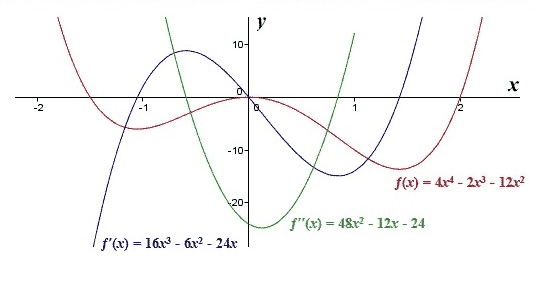
Graph of three curves over x from -2 to 2: f(x) = 4x^4 - 2x^3 - 12x^2 in red, f'(x) = 16x^3 - 6x^2 - 24x in dark blue, and f''(x) = 48x^2 - 12x - 24 in green, with labeled x and y axes.


Worked solution of dy/dx = x^2 - 3: both sides multiplied by dx giving dy = (x^2 - 3)dx, integrated to y = x^3/3 - 3x + K.


BvU said:
take ##f(x)= x^2-3## . Add initial condition f(0) = 0 so it yields a unique solution.

##x = 0 \rightarrow f(0) = 0##

##x = 0.1 \rightarrow f(0.1) = 0 + (0.01 - 3)* 0.1 = -0.299 \ ## exact solution ##f(0.1) = 0.001 - 3 = -0.299 \ ##

etc. etc.

we get:
Table comparing a numerical approximation with the exact solution at x = 0 to 1 in steps of 0.1, with columns for numerical value, exact value and error; the error grows from 0 to 0.6150 at x = 1.


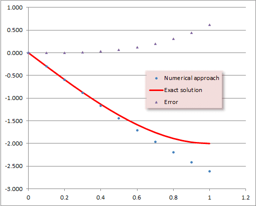
Scatter and line plot of a numerical approximation, the exact solution curve, and the error against x from 0 to 1.2; the exact solution curve falls from 0 to about -2 at x = 1.


So the exact solution is a function ##f(x) = x^3/3-3x## and the numerical approach is a table of aproximated function values.

(I took steps of 0.1 so the difference between exact and numerical becomes visible).

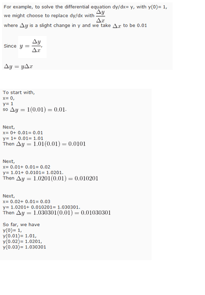
Handwritten-style worked example of Euler's method for dy/dx = y with y(0) = 1 and step size 0.01, showing steps x = 0, 0.01, 0.02, 0.03 and resulting y values 1, 1.01, 1.0201, 1.030301.


BvU said:
this differential equation does have a condition: ##f(0) = 1##. You solve numerically by approaching f(0) as a linear function for a small step:$$f(0+\Delta x) \approx f(0) + \Delta x {dy\over dx}$$ when all you really know is $$ \lim_{h\downarrow 0} {f(0+h) - f(0) \over h } = {dy\over dx} \ .$$
When you take a few steps you get a sequence of approximated function values, but not a function (in the sense of an exact prescription what to do with x to get y).

So for ##\ f(x)= y\ \ \& \ \ f(0) = 1 \ ## you have found four function values, not four functions.
So the exact solution is a function ##f(x) = x^3/3-3x## and the numerical approach is a table of approximated function values.

When you take a few steps you get a sequence of approximated function values, but not a function (in the sense of an exact prescription what to do with x to get y).

BvU said:
Yes. Note that replacing ##\ dy\over dx\ ## by ##\ \Delta y\over \Delta x\ ## is an approximation...
is this what we use the numerical methods for ?? to simply get approximated function values??
 
You are using the so-called Forward Euler finite difference approximation to carry out the numerical integration. This formula is only first order accurate in ##\Delta x##. There are higher order formulas that give much better accuracy. An example is the trapazoidal rule formula.
 
a question usually starts like this ...

find the function that gives , this instantaneous rate of change ...
Graph of three curves on x and y axes: f(x) = 4x^4 - 2x^3 - 12x^2 in red, f'(x) = 16x^3 - 6x^2 - 24x in blue, and f''(x) = 48x^2 - 12x - 24 in green.


Worked solution of dy/dx = x^2 - 3 by separation and integration: dy = (x^2 - 3)dx, integrated to y = x^3/3 - 3x + K, with explanatory text in between.

If the precise form of the function is not known it is better to construct an approximation using the methods like ,
Forward Euler finite difference
Trapazoidal rule formula.

so we only use numerical methods If the precise form of the function is not known ...
and with numerical methods ... we get function values ... right ??
 
rosekidcute said:
If the precise form of the function is not known it is better to construct an approximation using the methods like ,
Forward Euler finite difference
Trapazoidal rule formula.

so we only use numerical methods If the precise form of the function is not known ...
and with numerical methods ... we get function values ... right ??
I don't quite understand your question. Can you give some examples for each option.
 
OK let me re arrange it one more time ...
a question usually starts like this ...

find the function that gives , this instantaneous rate of change ...
Graph of three polynomial curves on x and y axes: f(x) = 4x^4 - 2x^3 - 12x^2 in red, f'(x) = 16x^3 - 6x^2 - 24x in blue, and f''(x) = 48x^2 - 12x - 24 in green, labelled on the plot.


Worked separation-of-variables example: dy/dx = x^2 - 3 becomes dy = (x^2 - 3)dx, integrated to give y = x^3/3 - 3x + K.


i don't understand the answer part properly ...

Text reading: That means that y(x) = x^3/3 - 3x + K has the property that for any value of K, at each value of x, the gradient, i.e. derivative with respect to x which is, indeed, the rate at which y is changing as x changing, is dy/dx = x^3 - 3


aren't we trying to find the precise form of the function , that gave us that instantaneous rate of change ...when do we use numerical methods ??

do we use it when the precise form of the function is not known ...If the precise form of the function is not known it is better to construct an approximation using the methods like ,
Forward Euler finite difference
Trapezoidal rule formula.

and with numerical methods ... we get function values ... right ??
 
Is your question, "Under what circumstances is numerical integration used to integrate a function or to solve a first order ordinary differential equation?"
 
yes , exactly ...

"Under what circumstances is numerical integration used to integrate a function or to solve a first order ordinary differential equation?"

Graph of f(x) = 4x^4 - 2x^3 - 12x^2 in red, with its derivative f'(x) = 16x^3 - 6x^2 - 24x in blue and second derivative f''(x) = 48x^2 - 12x - 24 in green, plotted against x from -2 to 2.

Worked solution of dy/dx = x^2 - 3 by separation: multiply by dx to get dy = (x^2 - 3)dx, integrate both sides, giving y = x^3/3 - 3x + K.


Text equation: y(x) = x^3/3 - 3x + K, with dy/dx = x^3 - 3, stated as the rate at which y changes as x changes.


BvU said:
Yes. Note that replacing ##\ dy\over dx\ ## by ##\ \Delta y\over \Delta x\ ## is an approximation...

Worked Euler method example for dy/dx = y with y(0) = 1 and step size 0.01, listing steps from x = 0 to x = 0.03 with the resulting values y(0.01) = 1.01, y(0.02) = 1.0201, y(0.03) = 1.030301.
BvU said:
Seems to me you still have trouble understanding what you did for ##y'=y## so let's step back and treat ##y'= x^2-3## the same way. Add initial condition y(0) = 0 so it yields a unique solution.

##x = 0 \rightarrow y(0) = 0##

##x = 0.1 \rightarrow y(0.1) = 0 + (0.01 - 3)* 0.1 = -0.299 \ ## exact solution ##y(0.1) = 0.001 - 3 = -0.299 \ ##

etc. etc.

we get:

Spreadsheet table comparing a numerical approach with an exact solution for x from 0 to 1 in steps of 0.1, with an error column that grows as x increases.


Line chart comparing a numerical approach (blue dots), the exact solution (red curve) and the error (purple triangles) for x from 0 to 1.2; the numerical points drift below the exact curve as x increases, and the error rises from 0 to about 0.6.


If the precise form of the function is not known it is better to construct an approximation using the methods like ,
Forward Euler finite difference
Trapazoidal rule formula.

so we only use numerical methods If the precise form of the function is not known ...
and with numerical methods ... we get function values ... right ??
 
Last edited:
i found some good notes online ...

http://calculuslab.deltacollege.edu/ODE/ODE-h.html

At this point in your differential equations course you should have gotten used to a few of the analytic techniques used to solve first order differential equations. The technique varies somewhat according to the form of the original equation, and you may already have seen forms classified as separable, exact, homogeneous, or linear. The method of solution of each of these forms inevitably involves some type of integration in order to eliminate the unwanted derivative.

For the most part the techniques can become rote exercises, whereby you, the student, classifies the form of the equation, then follows the appropriate recipe to solve it. This kind of repetition sounds like an ideal task for relegating to a computer.

Recall that when solving a differential equation alone we are typically led to a family of solutions, determined by the presence of one or more constants.

In order to narrow this infinity of solutions to a unique solution it is necessary to impose one or more initial conditions, depending on the order of the differential equation. When this is done we say that we are now working with a an initial value problem

We have learned theorems that guarantee to us that under the right conditions an initial value problem has a solution that both exists, and is unique on some interval containing the x-value in the initial condition(s). However, we have also seen that despite this guarantee, it is frequently impossible to actually find this solution by standard techniques.

We have learned theorems that guarantee to us that under the right conditions an initial value problem has a solution that both exists, and is unique on some interval containing the x-value in the initial condition(s). However, we have also seen that despite this guarantee, it is frequently impossible to actually find this solution by standard techniques.

What this usually means is that the solution we seek cannot be written in a form that uses a combination of the standard "elementary" mathematical functions that we are used to. This may come as a shock at first, but absolutely the same problem exists for the majority of functions you might sketch by randomly drawing a functional graph on a piece of paper. In fact we might state this fact even more strongly: The vast majority of functions from the univeral set of all possible functions cannot be described with a formula. It is not surprising then that so many differential equations have solutions that fit into this category.

So what then? Should we just banish these "impossible" differential equations from our consideration and pretend that they don't exist? That would be fine, but all too many of them are the very equations which describe "real life" physical phenomena. These are the differential equations we have to solve to model the heat flowing through a steel rod, or put a space shuttle into orbit. We can't just not solve them.

The somewhat unsatisfying truth is that we must find approximate numerical solutions to most actual applied differential equations. Now remember, these solutions will not be given by the kind of formulas we are used to. Rather, numerical solutions will be lists of points which lie, hopefully, close to the actual solution's curve.

Some numerical methods play "join the dots" with these points to mimic, as best they can, the behavior of the actual solution. One note about this kind of solution: it can't contain any arbitrary constants. We get one solution, not a family of solutions. This means that the problems we solve must be initial value problems

rosekidcute said:
yes , exactly ...

"Under what circumstances is numerical integration used to integrate a function or to solve a first order ordinary differential equation?"

Graph of three curves on x and y axes: f(x) = 4x^4 - 2x^3 - 12x^2 in red, f'(x) = 16x^3 - 6x^2 - 24x in blue, and f''(x) = 48x^2 - 12x - 24 in green, over x from -2 to 2.

Handwritten-style worked solution separating variables for dy/dx = x^2 - 3: multiply by dx to get dy = (x^2 - 3)dx, integrate to get y = x^3/3 - 3x + K.


Text explaining that y(x) = x^3/3 - 3x + K has, for any constant K, a gradient dy/dx = x^3 - 3, the rate at which y changes as x changes.


Worked example of Euler's method for dy/dx = y with y(0) = 1 and step size 0.01, showing steps x = 0 to 0.03 and values y(0.01) = 1.01, y(0.02) = 1.0201, y(0.03) = 1.030301.
Spreadsheet table comparing a numerical approach with an exact solution for x from 0 to 1 in steps of 0.1, with columns for x, numerical value, exact value and error.


Graph of a numerical approach to an ODE solution against the exact solution curve for x from 0 to 1.2, with the error plotted as triangles; points drift below the red curve as x increases.


If the precise form of the function is not known it is better to construct an approximation using the methods like ,
Forward Euler finite difference
Trapazoidal rule formula.

so we only use numerical methods If the precise form of the function is not known ...
and with numerical methods ... we get function values ... right ??
If the precise form of the function is not known it is better to construct an approximation using the numerical methods

how do i construct these approximations ...??
 
Last edited: