Undergrad Why is this Hubble plot linear for Omega=2 closed universe?

[Bandersnatch]

TL;DR

I'm trying to get an intuitive understanding of how different expansion models show up on the Hubble plot and I can't wrap my head around the linearity of this one.

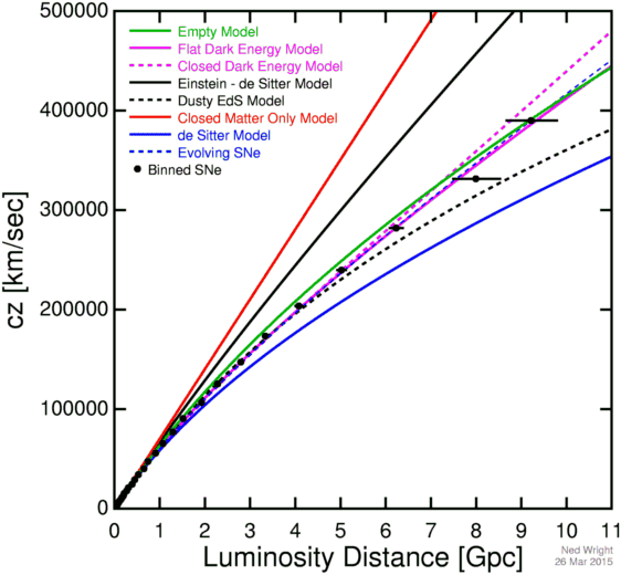
On Ned Wright's pages one can find this graph:

plotting some supernova data against different expansion models.
The main thing here that gives me a pause is the linear relationship for the closed universe with $\Omega$=2 (red line). There doesn't seem to be any weird scaling involved. What is it, then, about this particular density that makes the plot of redshift vs this particular distance measure linear?
A reference to a non-obscure textbook or an online resource should suffice and will be appreciated, but patient explanations are more than welcome.

 

[George Jones]

The main thing here that gives me a pause is the linear relationship for the closed universe with $\Omega$=2 (red line). There doesn't seem to be any weird scaling involved. What is it, then, about this particular density that makes the plot of redshift vs this particular distance measure linear? A reference to a non-obscure textbook or an online resource should suffice and will be appreciated, but patient explanations are more than welcome.

I can run through the math, but I can't give any real intuition for the $\Omega = 2$ matter-only case.

Below, I reference and use stuff from section 3.4 "Observations in Cosmology" in John Peacock's book "Cosmological Physics". This section is freely available on Ned Wright's website,
http://ned.ipac.caltech.edu/level5/Peacock/Peacock_contents.html
Equation (3.78),
$$R_0 S_k \left( r \right) = \frac{2c}{H_0}\frac{z \Omega + \left( \Omega - 2 \right) \left( \sqrt{1 + z \Omega} - 1\right)}{\Omega^2 \left( 1 + z \right)},$$
applies to a matter-dominated universe, and where $S_k \left( r \right)$ is the standard FLRW spatial metric given by (3.10)

When $\Omega = 2$, a crucial cancellation in the second term in the right numerator occurs, and this becomes
$$\begin{align}
R_0 S_k \left( r \right) &= \frac{2c}{H_0}\frac{z \Omega }{\Omega^2 \left( 1 + z \right)} \nonumber \\
&= \frac{c}{H_0}\frac{z}{1 + z} \nonumber .
\end{align} $$
Combining this with equation (3.91) for luminosity distance,
$$D_L = \left( 1 + z \right) R_0 S_k,$$
gives
$$D_L = \frac{cz}{H_0},$$
and
$$cz = H_0 D_L .$$
Hence, when $cz$ is plotted versus luminosity distance, the slope of the resulting straight line is
$$H_0 \approx 70 ~ \frac{\rm{km} / \rm{s}}{\rm{Mpc}} = 70000 ~\frac{\rm{km} / \rm{s}}{\rm{Gpc}},$$
which is consistent with values on the vertical and horizontal axes of the figure.