MHB Dale's questions via Facebook about Riemann Sums

[Prove It]

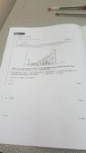
View attachment 7140
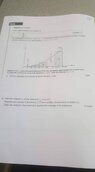
View attachment 7141

(a) Since a = 2, that means $\displaystyle \begin{align*} \Delta x = \frac{2}{5} \end{align*}$

(b)
$\displaystyle \begin{align*} f \left( \frac{7\,\Delta x}{2} \right) &= f \left( \frac{7}{5} \right) \\ &= \left( \frac{7}{5} \right) ^2 \\ &= \frac{49}{25} \end{align*}$

(c)
$\displaystyle \begin{align*} A_4 &= f \left( \frac{7}{5} \right) \cdot \Delta x \\ &= \frac{49}{25} \cdot \frac{2}{5} \\ &= \frac{98}{125} \,\textrm{units}^2 \end{align*}$

(d)
$\displaystyle \begin{align*} A_i &= f \left( x_i \right) \cdot \Delta x \end{align*}$

(e)
$\displaystyle \begin{align*} S_5 &= \sum_{i = 1}^5{ \left[ f \left( x_i \right) \cdot \Delta x \right] } \\ &= f \left( x_1 \right) \cdot \Delta x + f \left( x_2 \right) \cdot \Delta x + f \left( x_3 \right) \cdot \Delta x + f \left( x_4 \right) \cdot \Delta x + f \left( x_5 \right) \cdot \Delta x \\ &= \left( \frac{1}{5} \right) ^2 \cdot \frac{2}{5} + \left( \frac{3}{5} \right) ^2 \cdot \frac{2}{5} + \left( \frac{5}{5} \right) ^2 \cdot \frac{2}{5} + \left( \frac{7}{5} \right) ^2 \cdot \frac{2}{5} + \left( \frac{9}{5} \right) ^2 \cdot \frac{2}{5} \\ &= \frac{1}{25} \cdot \frac{2}{5} + \frac{9}{25} \cdot \frac{2}{5} + \frac{25}{25} \cdot \frac{2}{5} + \frac{49}{25} \cdot \frac{2}{5} + \frac{81}{25} \cdot \frac{2}{5} \\ &= \frac{2}{125} + \frac{18}{125} + \frac{50}{125} + \frac{98}{125} + \frac{162}{125} \\ &= \frac{330}{125} \\ &= \frac{66}{25} \,\textrm{units}^2 \end{align*}$

(f)
$\displaystyle \begin{align*} A &= \int_0^a{f\left( x \right) \,\mathrm{d}x} \\ &= \int_0^2{ x^2\,\mathrm{d}x } \\ &= \left[ \frac{x^3}{3} \right] _0^2 \\ &= \frac{2^3}{3} - \frac{0^3}{3} \\ &= \frac{8}{3} \,\textrm{units}^2 \end{align*}$

(g)
$\displaystyle \begin{align*} \textrm{Error} &= \frac{66}{25} - \frac{8}{3} \\ &= \frac{198}{75} - \frac{200}{75} \\ &= -\frac{2}{75} \end{align*}$

So the percentage error is

$\displaystyle \begin{align*} \frac{-\frac{2}{75}}{\frac{8}{3}} \cdot 100\% &= -\frac{2}{75} \cdot \frac{3}{8} \cdot 100\% \\ &= -\frac{600\%}{600} \\ &= -1\% \end{align*}$

 

[Prove It]

View attachment 7142

(a) Since the distance along the x-axis is "b" and it is being divided into "n" rectangles, that means $\displaystyle \begin{align*} \Delta x = \frac{b}{n} \end{align*}$.

(b) Each interval can be written as $\displaystyle \begin{align*} \left[ \left( i - 1 \right) \Delta x , i\,\Delta x \right] \end{align*}$, so that means the midpoint of each interval is

$\displaystyle \begin{align*} x_i &= \frac{\left( i - 1 \right) \Delta x + i\,\Delta x}{2} \\ &= \frac{\left( i - 1 + i \right) \Delta x}{2} \\ &= \frac{\left( 2\,i - 1 \right) \Delta x}{2} \end{align*}$

View attachment 7144

(c) Since we have found $\displaystyle \begin{align*} \Delta x = \frac{b}{n} \end{align*}$ that means

$\displaystyle \begin{align*} x_i &= \frac{\left( 2\,i - 1 \right) \Delta x}{2} \\ &= \frac{\left( 2\,i - 1 \right) \frac{b}{n}}{2} \\ &= \left( 2\,i - 1 \right) \frac{b}{2\,n} \end{align*}$

(d) The length of each rectangle is $\displaystyle \begin{align*} \Delta x \end{align*}$ and the width is $\displaystyle \begin{align*} g \left( x_i \right) \end{align*}$ so the area of each rectangle is $\displaystyle \begin{align*} A_i = g \left( x_i \right) \Delta x \end{align*}$

(e) Since $\displaystyle \begin{align*} x_i = \left( 2\,i - 1 \right) \frac{b}{2\,n} \end{align*}$ that means $\displaystyle \begin{align*} g \left( x_i \right) = g \left( \left( 2\,i - 1 \right) \frac{b}{2\,n} \right) \end{align*}$ and $\displaystyle \begin{align*} \Delta x = \frac{b}{n} \end{align*}$ that means $\displaystyle \begin{align*} g \left( \left( 2\,i - 1 \right) \frac{b}{2\,n} \right) \frac{b}{n} = g \left( x_i \right) \Delta x \end{align*}$, so

$\displaystyle \begin{align*} \sum_{i = 1}^n{ \left[ g\left( \left( 2\,i - 1 \right) \frac{b}{2\,n}\right) \Delta x \right] } &= \sum_{i = 1}^n{ \left[ g \left( x_i \right) \Delta x \right] } \\ &= \sum_{i = 1}^n{A_i} \end{align*}$

(f) (i) If $\displaystyle \begin{align*} g \left( x \right) = x^3 \end{align*}$, that means

$\displaystyle \begin{align*} \sum_{i = 1}^n{ A_i } &= \sum_{i = 1}^n{ \left[ g \left( \left( 2\,i - 1 \right) \frac{b}{2\,n} \right) \Delta x \right] } \\ &= \sum_{i = 1}^n{ \left\{ \left[ \left( 2\,i - 1 \right) \frac{b}{2\,n} \right] ^3 \,\frac{b}{n} \right\} } \end{align*}$

so when $\displaystyle \begin{align*} n = 100 \end{align*}$ we have

$\displaystyle \begin{align*} \sum_{i = 1}^{100}{ \left\{ \left[ \left( 2\,i - 1 \right) \frac{b}{100}\right] ^3\,\frac{b}{100} \right\} } &= \frac{19\,999\,b^4}{80\,000} \end{align*}$

Wolfram|Alpha: Computational Knowledge Engine

(ii)
$\displaystyle \begin{align*} A &= \lim_{n \to \infty}{ \left\{ \left[ \left( 2\,i - 1 \right) \frac{b}{n} \right] ^3 \,\frac{b}{n} \right\} } \\ &= \frac{b^4}{4} \end{align*}$

Wolfram|Alpha: Computational Knowledge Engine

View attachment 7145(g) The exact area under the curve $\displaystyle \begin{align*} g(x) = x^3 \end{align*}$ between x = 0 and x = b is

$\displaystyle \begin{align*} A &= \int_0^b{x^3\,\mathrm{d}x} &= \left[ \frac{x^4}{4} \right] _0^b \\ &= \frac{b^4}{4} - \frac{0^4}{4} \\ &= \frac{b^4}{4} \,\textrm{units}^2 \end{align*}$

(i) so the error in using 100 rectangles for the approximation is

$\displaystyle \begin{align*} \frac{b^4}{4} - \frac{19\,999\,b^4}{80\,000} &= \frac{20\,000\,b^4}{80\,000} - \frac{19\,999\,b^4}{80\,000} \\ &= \frac{b^4}{80\,000} \end{align*}$

and so the percentage error is

$\displaystyle \begin{align*} \frac{\frac{b^4}{80\,000}}{\frac{b^4}{4}} \cdot 100\% &= \frac{b^4}{80\,000} \cdot \frac{4}{b^4} \cdot 100\% \\ &= \frac{100\%}{20\,000} \\ &= 0.005\% \end{align*}$

(ii) and as the limiting value is exactly equal to the integral value, the percentage error is 0%.