Diff eqs with eigenvectors: double roots, but 2nd eigenvector?

Join the discussion
Ask a follow-up here, or get your own question answered by working scientists, mathematicians and engineers — people, not an autocomplete.
Real named experts · corrections over time · the nuance an AI answer skips
9 replies · 2K views
kostoglotov
Messages
231
Reaction score
6
The problem is here, I'm trying to solve (b):
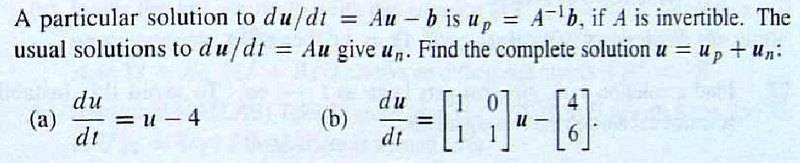
ifVm57o.jpg


imgur link: http://i.imgur.com/ifVm57o.jpg

and the text solution is here:

qxPuMpu.png


imgur link: http://i.imgur.com/qxPuMpu.pngI understand why there is a term in there with [itex]cte^t[/itex], it's because the A matrix has double roots for the eigenvalues. What I don't understand is where the (apparent) second eigenvector, [itex] \begin{bmatrix}1\\ t\end{bmatrix}[/itex] is coming from?

I gave my answer as [itex]\vec{u} = \begin{bmatrix}4\\ 2\end{bmatrix} + c_1e^t\begin{bmatrix}0\\ 1\end{bmatrix}+c_2te^t\begin{bmatrix}0\\ 1\end{bmatrix}[/itex].

This answer works, but so does the text answer, and it is more complete. But where did that second distinct eigenvector come from?
 
Physics news on Phys.org
kostoglotov said:
This answer works, but so does the text answer, and it is more complete. But where did that second distinct eigenvector come from?
You have a double eigenvalue ##\lambda = 1## with geometric multiplicity one, giving you one eigenvector ##v_1 = (0,1)##, and algebraic multiplicity two. So, in order to span the generalised eigenspace corresponding to ##\lambda## (which is just ##\mathbb{R}^2##) you need a generalised eigenvector ##v_2##, which you can obtain by solving
$$
Av_2 = \lambda v_2 + v_1
$$
(The sequence ##\{v_1,v_2\}## is called a Jordan chain corresponding to ##\lambda## and ##v_1##.) Then the solution to the homogeneous system is
$$
u_n(t) = c_1 e^{\lambda t}v_1 + c_2 t e^{\lambda t}v_2
$$
You can see that your own solution is not the most general one, because at time ##t = 0## you cannot satisfy an arbitrary initial condition. (In fact, as you can see you can only satisfy initial conditions ##u_0## for which ##u_0 - (4,2)## is in the span of ##(0,1)##.) This is because ##v_1## by itself does not span the generalised eigenspace.
 
  • Like
Likes   Reactions: kostoglotov
A different approach from the one Krylov took...
Since it is straightforward to get a particular solution to the nonhomogeneous problem, let's look only at the homogeneous system:
##\vec{u}' = A\vec{u}##
This system has a solution ##\vec{u} = e^{At}C##, where C is a column matrix of coefficients that depend on initial conditions.

To calculate ##e^{At}##, we'll need to calculate the various powers of A.
##A = \begin{bmatrix} 1 & 0 \\ 1 & 1 \end{bmatrix}##
##A^2 = \begin{bmatrix} 1 & 0 \\ 2 & 1 \end{bmatrix}##
##A^3 = \begin{bmatrix} 1 & 0 \\ 3 & 1 \end{bmatrix}##
In general, ##A^n = \begin{bmatrix} 1 & 0 \\ n & 1 \end{bmatrix}##
If necessary, this last statement is easy to prove.

##e^{At} = I + At + \frac{A^2t^2}{2!} + \dots + \frac{A^nt^n}{n!} + \dots##
##= \begin{bmatrix} 1 & 0 \\ 0 & 1 \end{bmatrix} + t\begin{bmatrix} 1 & 0 \\ 1 & 1 \end{bmatrix} + \frac{t^2}{2!}\begin{bmatrix} 1 & 0 \\ 2 & 1 \end{bmatrix} + \dots + \frac{t^n}{n!}\begin{bmatrix} 1 & 0 \\ n & 1 \end{bmatrix} + \dots##
##= \begin{bmatrix} 1 + t + \frac{t^2}{2!} + \dots + \frac{t^n}{n!} + \dots & 0 \\ 0 + t + \frac{2t^2}{2!} + \dots + \frac{nt^n}{n!} + \dots & 1 + t + \frac{t^2}{2!} + \dots + \frac{t^n}{n!} + \dots \end{bmatrix}##
##= \begin{bmatrix} e^t & 0 \\ te^t & e^t \end{bmatrix}##
##= e^t\begin{bmatrix} 1 & 0 \\ t & 1 \end{bmatrix}##
In the matrix a couple of lines up, the expression in the lower left corner is just tet.

So the solution to the homogeneous problem, ##u_h(t)##, is ##u_h(t) = e^t\begin{bmatrix} 1 & 0 \\ t & 1 \end{bmatrix}C##,
or, ##u_h(t) = c_1e^t\begin{bmatrix} 1 \\ t \end{bmatrix} + c_2e^t\begin{bmatrix} 0 \\ 1 \end{bmatrix}##
In this last form, the two linearly independent eigenvectors are shown.
 
  • Like
Likes   Reactions: kostoglotov
Krylov said:
Then the solution to the homogeneous system is
$$
u_n(t) = c_1 e^{\lambda t}v_1 + c_2 t e^{\lambda t}v_2 \qquad (*)
$$
Mark44 made me realize that I made a mistake in this line yesterday, my apologies. The method is fine, though. From the Jordan chain you build the correct solution to the homogeneous equation as
$$
u_n(t) = c_1e^{\lambda t}v_1 + c_2e^{\lambda t}(v_2 + t v_1)
$$
I'm sorry for any confusion that I may have caused.
 
To make you see the pattern of constructing solutions using Jordan chains more clearly, I will add one example. Suppose you have the homogeneous ##3 \times 3## system corresponding to the matrix
$$
A =
\begin{bmatrix}
1& 0& 0\\
1& 1& 0\\
1& 1& 1
\end{bmatrix}
$$
You can check that ##\lambda = 1## is a triple eigenvalue of geometric multiplicity one. The lone eigenvector is given by ##v_1 = (0,0,1)##. To get the first generalised eigenvector, solve
$$
A v_2 = \lambda v_2 + v_1
$$
to obtain ##v_2 = (0,1,0)##. Similarly, to get the second generalised eigenvector, solve
$$
A v_3 = \lambda v_3 + v_2
$$
to obtain ##v_3 = (1, -1, 0)##. (There is not really a need for Gaussian elimination for these systems: you can find the solutions by inspection.) Then construct the solution as
$$
u_h(t) = c_1 e^{\lambda t} v_1 + c_2 e^{\lambda t}\Bigl(v_2 + \frac{t}{1!}v_1\Bigr) + c_3 e^{\lambda t}\Bigl(v_3 + \frac{t}{1!} v_2 + \frac{t^2}{2!}v_1\Bigr)
$$
where the ##c_i## are constants determined by your initial condition.

In my opinion, taking the matrix exponential directly (as in @Mark44 's post) is faster when it is easy to spot a general formula for the powers of ##A##. This is not always the case, in which instance you can rely on computing Jordan chains.
 
  • Like
Likes   Reactions: kostoglotov
In addition to the technique of calculating ##e^{At}## using powers of A, there's another technique that uses the Cayley-Hamilton theorem, which says that every matrix is a root of its characteristic equation. This technique appears in a Linear Algebra textbook I've hung onto, "Linear Algebra and Differential Equations," by Charles G. Cullen. Cullen's explanation isn't clear to me, so when I figure out what he's doing, I'll post an explanation using that technique.
 
  • Like
Likes   Reactions: kostoglotov
Krylov said:
you can find the solutions by inspection.

But by inspection you can see that there are multiple solutions to those equations for the generalized eigenvectors. [itex](0,1,1)[/itex] would work just as well to solve [itex](A-\lambda I)v_2 = v_1[/itex].
 
So here's the other method I mentioned in my previous post. The technique is presented in "Linear Algebra and Differential Equations," by Charles G. Cullen.

We're solving the DE ##\frac{d \vec{u}}{dt} = A \vec{u}##, or ##(D - A)\vec{u} = 0##, for which the solution is ##\vec{u} = e^{At}C##, where A and C are matrices.
For the problem at hand, ##A = \begin{bmatrix} 1 & 0 \\ 1 & 1\end{bmatrix}##

As was already mentioned in this thread, the matrix A has only one eigenvalue: ##\lambda = 1##.
The characteristic polynomial for the matrix is ##c(x) = (x = 1)^2 = x^2 - 2x + 1##, which is found by evaluating det(##\lambda##I - A).

For a diff. equation ##(D - 1)^2y = 0##, we would expect a solution of the form ##y = c_1 e^t + c_2te^t##.

Per a theorem by Ziebur, cited on page 307 of this textbook, "Every entry of ##e^{At}## is a solution of the nth-order equation c(D)y = 0, where c(x) = det(xI - A) is the characteristic polynomial of A."

That is, ##e^{At} = E_1e^t + E_2te^t##, where ##E_1## and ##E_2## are matrices of constants.

At t = 0, the equation above results in ##I = E_1##
Differentiating the equation above results in ##Ae^{At} = E_1e^t + E_2e^t + E_2te^t##
At t = 0, we have ##A = E_1 + E2##

Substituting I for ##E_1## and solving the second equation, we have ##E_2 = A - I = \begin{bmatrix} 0 & 0 \\ 1 & 0\end{bmatrix}##

Therefore, ##e^{At} = \begin{bmatrix} 1 & 0 \\ 0 & 1\end{bmatrix}e^t + \begin{bmatrix} 0 & 0 \\ 1 & 0\end{bmatrix}te^t##
##= \begin{bmatrix} 1 & 0 \\ t & 1\end{bmatrix}e^t = e^{At}##
Note that the columns of this last matrix hold the two linearly independent eigenvectors.
 
Last edited:
kostoglotov said:
But by inspection you can see that there are multiple solutions to those equations for the generalized eigenvectors ##(0,1,1)## would work just as well to solve ##(A-\lambda I)v_2 = v_1##.
True, you could equally well work with that choice for ##v_2##, but for the same initial condition ##u_0## as before the arbitrary coefficients ##c_i## would then be different and you would end up with exactly the same solution ##u_h## satisfying ##u_h(0) = u_0##.

(Note that once you make a different choice for ##v_2##, your solution for ##v_3## will also change.)
 
Last edited:
  • Like
Likes   Reactions: kostoglotov