Find the center manifold of a 2D system with double zero eigenvalues

[NicolaiTheDane]

TL;DR

A theorem on local center manifolds in my textbook, seems to suggest that my center manifold is 2D, but as the system itself is 2D, this does not make sense to me. I need some help to understand how to apply the theorem, or understand why I cannot.

I have to find the center manifold of the following system

\begin{align}
\dot{x}_1&=x_2 \\
\dot{x}_2&=-\frac{1}{2}x_1^2
\end{align}

which has a critical point at $x_0=\begin{bmatrix}0 & 0\end{bmatrix}$. Its linearization at that point is
\begin{align}
D\mathbf {f}(\mathbf {x_0}) = \begin{bmatrix}
0 & 1 \\
0 & 0
\end{bmatrix}
\end{align}
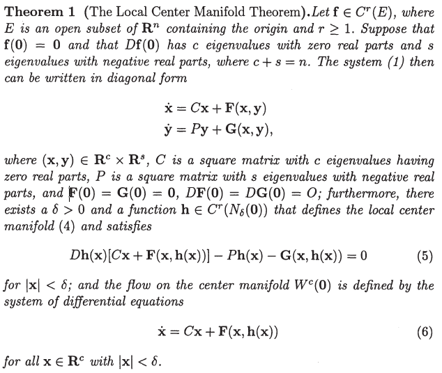
which obviously has the eigenvalue $\lambda = 0$, with the eigenvector $\mathbf{v}=\begin{bmatrix}1 & 0 \end{bmatrix}^T$. In the book (Differential Equations and Dynamical Systems 7. edition, by Perko) we are using in my introductory course on dynamical systems, we have the following theorem

We are advised to use polynomial approximations to find $h(x)$. However, since s = 0 (both eigenvalues are 0 exactly) I don't know how to utilize the theorem. With $c = n$ it would seem as though $P$ and $G$ has a dimensionality of 0, and $C$ is a 2 by 2 matrix with just zeros in it, effectively making $\mathbf {F}=D\mathbf {f}$. Another big problem is that this means $h$ is 2D and not 1D as would seem intuitive (since the geometric multiplicty of $\lambda=0$ is 1), and that obviously does not make sense, as the system itself is 2D. Can someone perhaps see where I'm going wrong here? I suspect that the theorem simply doesn't work for this case, and that it is missing the condition that $s \geq 1$, but its just a hunch.

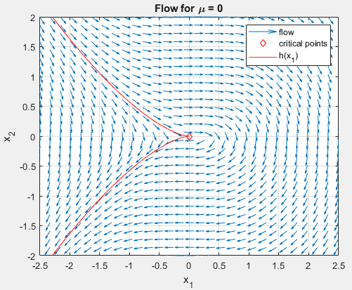
It should be said that some guess work has lead me to a function
\begin{align}
\dot{x}_2 = h(x_1) = \sqrt{-\frac{1}{3}x_1^3 + c}
\end{align}
where $c = 0$ so as to make it fit with the critical point. This seems to visually to do exactly what I want it to

Not sure this helps, but I thought I'd add it.

 

[pasmith]

The quantity E = x_2^2 + \frac13x_1^3 is conserved on every trajectory. Thus you are constrained to a one-dimensional manifold from the outset. Only in the case E = 0 does that manifold intersect the origin, thus making it "the centre manifold".

 

[NicolaiTheDane]

The quantity E = x_2^2 + \frac13x_1^3 is conserved on every trajectory. Thus you are constrained to a one-dimensional manifold from the outset. Only in the case E = 0 does that manifold intersect the origin, thus making it "the centre manifold".

The point of the centre manifold theorem is that you look to the centre manifold to tell you about the long-term behaviour of the system, but here that doesn't help you: you don't get closer to the centre manifold if you don't actually start on it.

So the theorem isn't applicable? The assignment suggests that if I were to use the theorem it would naturally lead me to a $h$ on the form $x_1=h_c(x_2)$. However, I don't see how this theorem does that. Keep in mind, I'm only on an introductory course, so you might have to be a bit more explanatory then average.

 

[pasmith]

Applying the theorem as stated would lead you to conclude that the center manifold is \mathbb{R}^2, and that the dynamics on the centre manifold are governed by a system which is the system you started with, <br /> \dot{\mathbf{x}} = C\mathbf{x} + \mathbf{F}(\mathbf{x}) = \begin{pmatrix} 0 &amp; 1 \\ 0 &amp; 0 \end{pmatrix}\mathbf{x} + \begin{pmatrix} 0 \\ -\frac12 x_1^2 \end{pmatrix}. So it does work; it just doesn't help you.

What is the exercise you are working on actually asking you to do with this system?

 

[NicolaiTheDane]

Applying the theorem as stated would lead you to conclude that the center manifold is \mathbb{R}^2, and that the dynamics on the centre manifold are governed by a system which is the system you started with, <br /> \dot{\mathbf{x}} = C\mathbf{x} + \mathbf{F}(\mathbf{x}) = \begin{pmatrix} 0 &amp; 1 \\ 0 &amp; 0 \end{pmatrix}\mathbf{x} + \begin{pmatrix} 0 \\ -\frac12 x_1^2 \end{pmatrix}. So it does work; it just doesn't help you.

What is the exercise you are working on actually asking you to do with this system?

As I suspected. The assignment itself simply says to assume
\begin{align}
x_2 = h(x_1)
\end{align}
and then find $h(x_1)$, which I have done with (4) by
\begin{align}
\dot{x}_2 = h'(x_1)\dot{x}_1 = -\frac{1}{2}x_1^2 \rightarrow \\
h'(x_1)x_2 = -\frac{1}{2}x_1^2 \rightarrow \\
h'(x_1)h(x_1) = -\frac{1}{2}x_1^2 \rightarrow \\
h'(x_1) = -\frac{1}{2h(x_1)}x_1^2
\end{align}
and solving the ODE getting (4), and concluding $c=0$ by
\begin{align}
h(0) = \pm\sqrt{c}=0
\end{align}
The problem I was having, was that the professor made a note in the assignment saying, that were I to use the theorem shown early instead, it would naturally lead to the assumption
\begin{align}
x_1 = h(x_2).
\end{align}
I simply couldn't (and still can't) figure out, how that theorem would lead me to that. It wasn't so much that I needed the help for the assignment itself (unless I'm completely off, but then that is too late now anyway, as I handed it in yesterday), as much as I needed help understanding how that theorem could have possible gotten me there, with this particular system.