roam
- 1,265
- 12
I am trying to implement several filters in Matlab for Fourier domain filtering. They are the cosine, Shepp-Logan, and Hann/Hamming window filters. These filters are defined as multiplying the ramp filter by the cosine function, sinc function, and Hann/Hamming windows respectively.
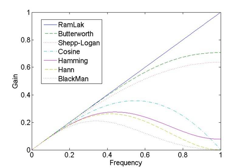
This is how the responses of these filters should look like:
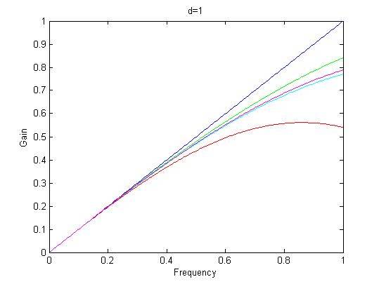
However, this is what I am getting:
I have defined the filters exactly as they are defined in this Matlab function, with a parameter ##d## that stretches the filters:
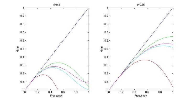
For instance, if I change it to ##d=0.3##, the Hann/Hamming filters start to look correct. And at ##d=0.65##, the cosine filter looks more correct:
So, what is the justification for using the parameter ##d##? And is there an algorithm for calculating it accurately for each filter?
Any explanation would be greatly appreciated.
This is how the responses of these filters should look like:
However, this is what I am getting:
Code:
w=linspace(0, 1, 181).'; % Frequency axis

d=0.33;

Hr = abs(w); % Ramp filter

H=Hr.* cos(w/(d)); % Cosine filter
H(H<0) = 0;

H=Hr.* (sin(w/d)./(w/d)); % Shepp-Logan filter
H(H<0) = 0;

H=Hr.* (1+cos(w./d)) / 2; % Hann filter
H(H<0) = 0;

H=Hr.* (.54 + .46 * cos(w/d)); % Hamming filter
H(H<0) = 0;
For instance, if I change it to ##d=0.3##, the Hann/Hamming filters start to look correct. And at ##d=0.65##, the cosine filter looks more correct:
So, what is the justification for using the parameter ##d##? And is there an algorithm for calculating it accurately for each filter?
Any explanation would be greatly appreciated.
