Undergrad Heat Equation: Solve with Non-Homogeneous Boundary Conditions

[erobz]

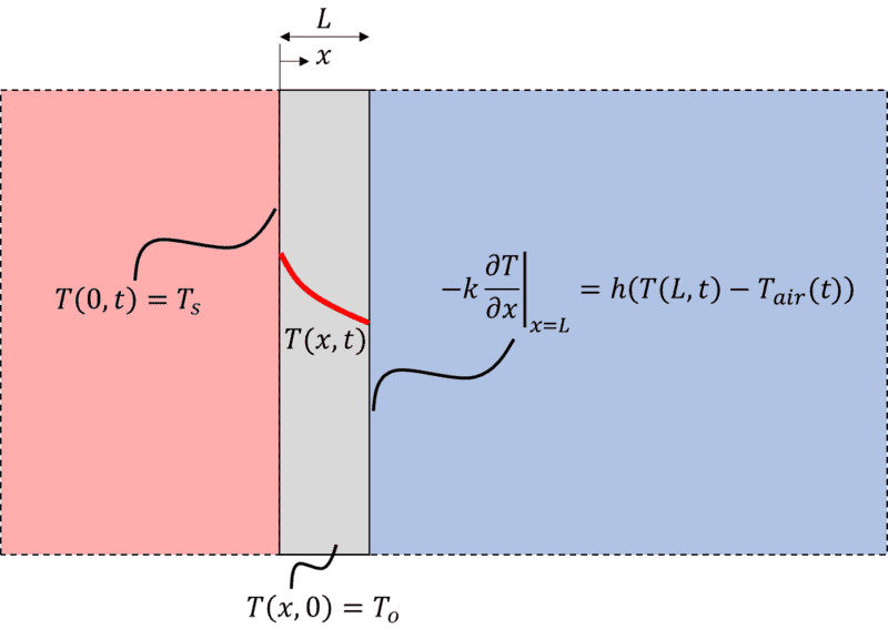
Imagine you have a plane wall with constant thermal conductivity, that is the intermediate between two thermal reservoirs:

The reservoir on the left is being kept at temp $T_s$, and it is a fluid that has very high convective coefficient $h$. As a result, the boundary condition at the LHS wall is given by:

$$ T(0,t) = T_s $$

at time $t=0$ the wall and the cold reservoir are brought into thermal contact with the warm reservoir. The wall and the blue reservoir are both initially at the same uniform temperature $T(x,0) = T_o$.

The blue reservoir and the wall start to heat up. The boundary condition on the RHS wall is given by:

$$ -k \left. \frac{\partial T}{ \partial x} \right|_{L} = h \left( T(L,t) - T_{air}(t) \right) $$

The heat equation for the plane wall is given by:

$$ \frac{\partial^2 T}{\partial x ^2} = \rho c_p \frac{\partial T}{\partial t}$$

So we have three non-homogenous boundary conditions, what is the idea to solve the PDE? Apparently, separation of variables does not work because of the non-zero boundary conditions.

The only thing I know (almost nothing) about solving PDE's I've learned from YouTube videos... Why does having non-zero boundary conditions throw a fork in it, and how big of a fork is it?

Thanks for any guidance!

 

[pasmith]

What do we know about T_{\mathrm{air}}?

Have you tried a Laplace transform in time? That gives <br /> \kappa(p\hat T - T_0) = \frac{\partial^2 \hat T}{\partial x^2} where \kappa= \rho c_p subject to <br /> \hat T(0,p) = \frac{T_s}{p}, \quad \left.-k\frac{\partial \hat T}{\partial x}\right|_{x=L} = h(\hat T(L,p) - \hat T_{air}(p)). That does leave you with <br /> \hat T(x,p) = \frac{T_0}{p} + A(p)\cosh(\sqrt{\kappa p}x) + B(p)\sinh(\sqrt{\kappa p}x) which is not easy to invert.

 

[erobz]

What do we know about T_{\mathrm{air}}?

It's going to be found via the following ODE:

$$ m_{air} c_{air} \frac{dT_{air}}{dt} = h A ( T(L,t) - T_{air}(t) ) + \dot q \tag{2}$$

The first term on the RHS is basically the boundary condition on the right wall. The $\dot q$ is just a constant term.

Have you tried a Laplace transform in time? That gives <br /> \kappa(p\hat T - T_0) = \frac{\partial^2 \hat T}{\partial x^2} where \kappa= \rho c_p subject to <br /> \hat T(0,p) = \frac{T_s}{p}, \quad \left.-k\frac{\partial \hat T}{\partial x}\right|_{x=L} = h(\hat T(L,p) - \hat T_{air}(p)). That does leave you with <br /> \hat T(x,p) = \frac{T_0}{p} + A(p)\cosh(\sqrt{\kappa p}x) + B(p)\sinh(\sqrt{\kappa p}x) which is not easy to invert.

I'm not lying when I said the only thing I know about PDE methods is from YouTube. Heck, I have very little formal understanding of ODE's for that matter. Am I understanding correctly that separation of variables simply does not work. Or is it that it takes extra massaging?

I was hoping that if I could find $T(x,t) = F(x)G(t)$, then I could use:

$$ \left. \frac{\partial T}{ \partial x} \right|_{x=L} = \left. \frac{\partial F}{ \partial x} \right|_{x=L} G(t) $$

subbing into (2) to get some kind of system.

I'm likely just getting all tangled up in stuff that won't work.

 

[erobz]

Have you tried a Laplace transform in time? That gives <br /> \kappa(p\hat T - T_0) = \frac{\partial^2 \hat T}{\partial x^2} where \kappa= \rho c_p subject to <br />

<br /> How does this work? I see you have introduced $p$ and the partial w.r.t. time disappears? I’m obviously oblivious to something.

 

[Chestermiller]

What do we know about T_{\mathrm{air}}?

In this context, $T_{air}$ is considered the bulk air temperature outside the thermal boundary layer.