How to transform a plot to use a logarithmic scale?

Click For Summary
SUMMARY

This discussion focuses on transforming a plot to a logarithmic scale using MATLAB. The user initially fits a model to simulated data generated by the equation y = a*exp(-t/b) + c, incorporating noise. They explore whether to convert y-values to log-scale before fitting, ultimately discovering that using MATLAB's built-in axis properties to set YScale to 'log' is a more effective approach, avoiding the need for manual logarithmic transformations.

PREREQUISITES
  • Familiarity with MATLAB programming and syntax
  • Understanding of exponential functions and their properties
  • Knowledge of curve fitting techniques, specifically using lsqcurvefit
  • Basic concepts of logarithmic scales and their applications in data visualization
NEXT STEPS
  • Learn how to use MATLAB's axis properties to manipulate plot scales, specifically the YScale property
  • Explore the effects of logarithmic transformations on data fitting and model accuracy
  • Investigate the implications of using different logarithmic bases (e.g., natural log vs. base 10)
  • Study advanced curve fitting techniques in MATLAB, including weighted fitting methods
USEFUL FOR

Data scientists, MATLAB users, and researchers involved in data analysis and visualization who seek to enhance their understanding of logarithmic transformations and their impact on data fitting.

Leonid92
Messages
45
Reaction score
2
I wrote the following code in MATLAB:
Code:
t = [0:0.001:0.1];
noise = randn(1,size(t,2));
a = 15*10^9;
b = 15*10^(-3);
c = 7*10^8;
y = a*exp(-t/b)+c+noise*100000000;
fun = @(p,t)p(1)*exp(-t/p(2))+p(3);
p0 = [15.5*10^9, 14*10^(-3), 6*10^8];
p = lsqcurvefit(fun, p0, t, y);
t_fit = [0:0.0001:0.1];
y_fit = fun(p,t_fit);
fig = figure('Visible','on');
plot(t,y,'.');
hold on;
grid on;
plot(t_fit,y_fit,'r','linewidth',2);
disp(sprintf('a=%d; b=%.4f; c=%d',p(1),p(2),p(3)))
Thus I generated data whose behavior is described by equation y = a*exp(-t/b)+c, with adding some noise. Then I fit mentioned function to these data and found values of parameters:
Code:
a=1.550000e+10; b=0.0149; c=6.000000e+08
The plot of simulated data and fit is below:
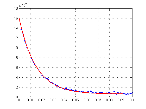
plot-exp.png

One person told me that it would be good to consider this problem in logarithmic scale. Could you please tell me, what is usually implied when talking about transforming ordinary plot to logarithmic scale? How should I implement this procedure? Should I first convert my simulated y-values into log-scale and after that perform fit with another function? What formulas should I use? Is it reasonable to use logarithm with base 10 or logarithm with base 'e'?
I will be very appreciate for any help or advice.
P.S. Unfortunately, I don't have opportunity to ask that person in more detail regarding this question.
 

Attachments

  • plot-exp.png
    plot-exp.png
    2.7 KB · Views: 1,824
Physics news on Phys.org
solve for t, it took me two lines, it is easily found.
 
  • Like
Likes   Reactions: Leonid92
Dr Transport said:
solve for t, it took me two lines, it is easily found.
You mean
Code:
b*ln( (y-c)/a ) = -t
?
I don't understand. I have simulated data and need to convert y-values to log-scale. Should I just take logarithm(y) ?
 
Have you tried substituting log(y_fun) for y_fun in the plot() line?
 
  • Like
Likes   Reactions: Leonid92
jedishrfu said:
Have you tried substituting log(y_fun) for y_fun in the plot() line?

In my code, I changed two lines:
Code:
plot(t,log(y),'.');
plot(t_fit,log(y_fit),'r','linewidth',2);
And the plot is:
plot-exp1.png

But I have doubt, is it right? I mean, is this what I need? What is the sense in this operation? I thought that firstly I should convert simulated y-values to log-scale, and then perform fitting with new, logarithmic function - fit logarithmic function to transformed y-values, is it right?
 

Attachments

  • plot-exp1.png
    plot-exp1.png
    3 KB · Views: 1,181
I tried the following:
Code:
t = [0:0.001:0.1];
noise = randn(1,size(t,2));
a = 15*10^9;
b = 15*10^(-3);
c = 7*10^8;
y = a*exp(-t/b)+c+noise*100000000;
y = log(y); % here is the change!
fun = @(p,t)log(p(1)*exp(-t/p(2))+p(3)); % here is the change!
p0 = [15.5*10^9, 14*10^(-3), 6*10^8];
p = lsqcurvefit(fun, p0, t, y);
t_fit = [0:0.0001:0.1];
y_fit = fun(p,t_fit);
fig = figure('Visible','on');
plot(t,y,'.');
hold on;
grid on;
plot(t_fit,y_fit,'r','linewidth',2);
disp(sprintf('a=%d; b=%.4f; c=%d',p(1),p(2),p(3)))

The plot is:
plot-exp2.png

I.e. firstly I converted simulated y-values to ln(y), and then performed fitting with function log( a*exp(-t/b)+c ), and it is seen that fit is not good.
Found parameters in this case are the following:
Code:
a=1.550000e+10; b=0.0156; c=6.000001e+08
So for me, transition to log-scale doesn't make sense.
 

Attachments

  • plot-exp2.png
    plot-exp2.png
    3 KB · Views: 1,090
Problem being the constant present, and the weights of the individual points. In the normal fit the points values had equal weights. In the fit of the log the low values get disproportional weights.
 
  • Like
Likes   Reactions: Leonid92

Similar threads

  • · Replies 2 ·
Replies
2
Views
4K
  • · Replies 12 ·
Replies
12
Views
4K
  • · Replies 6 ·
Replies
6
Views
4K
Replies
2
Views
3K
  • · Replies 1 ·
Replies
1
Views
4K
  • · Replies 14 ·
Replies
14
Views
4K
  • · Replies 4 ·
Replies
4
Views
2K
  • · Replies 18 ·
Replies
18
Views
4K
  • · Replies 1 ·
Replies
1
Views
3K
  • · Replies 7 ·
Replies
7
Views
3K