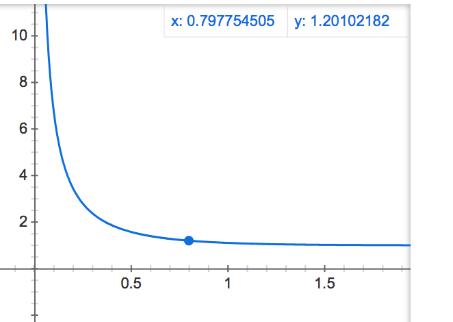
Hubble Parameter as function of time in universe models

[timmdeeg]

This graph shows $H$ as a function of time related to the L-CDM model. Do we (@Jorrie) have similar graphs e.g. for $\Lambda=0$; $k=-1$ critical, $\Lambda=0$; $k=0$ open, $\Lambda=0$; $k=+1$ closed?

That would be great, thanks in advance.

 

[Jorrie]

Not precisely, but you can get close enough for all practical purposes by playing around with the input parameters and output options. E.g. $\Lambda = 0.0000001$, set the output scaling to Normalized, select Chart and set hor and vert scales appropriately:

For Open and Closed cases, you play around with $\Omega$. I have used the http://jorrie.epizy.com/docs/index.html?i=1 version, which has more liberal range limits than the approved Github version.

 

[timmdeeg]

Ah, great, thanks for your advise!

One question, how can I show only one of these curves?

 

[Jorrie]

Just go to 'Column definition and selection'. I usually click 'none' and then select the two or three that I need. The default selections are just to give an idea of how it works.

 

[timmdeeg]

Got it, thanks.

 

[Bandersnatch]

@Jorrie is there a way for the calculator to show recollapse? I can't seem to get there no matter how I fiddle with the parameters.

 

[Jorrie]

Lightcone8 does not allow for high Omega or very small Lambda, so I'm not sure that collapse can happen with these limitations. Any small Lambda may quickly become dominant again.
As a matter of fact it seems to crash if I set Lambda to 0.001 and Omega to 1.5. Will have to investigate that.

I recall that I have previously simulated a zero lambda situation with collapse on older, less accurate versions, but it will take some searching to find that.

 

[George Jones]

This graph shows $H$ as a function of time related to the L-CDM model. Do we (@Jorrie) have similar graphs e.g. for $\Lambda=0$; $k=-1$ critical, $\Lambda=0$; $k=0$ open, $\Lambda=0$; $k=+1$ closed?

@Jorrie is there a way for the calculator to show recollapse?

In a closed matter-only (dust) FLRW univers, parametric expessions for the scale factor $a$ and cosmological time $t$ as functions of conformal time $η$ are (from Ryden)
$$\begin{align}
a\left(\eta\right) &= \frac{1}{2} \frac{\Omega_0}{\Omega_0 - 1} \left( 1 - \cos\eta \right) \\
t\left(\eta\right) &= \frac{1}{2H_0} \frac{\Omega_0}{\left( \Omega_0 - 1 \right)^{3/2}} \left( \eta - \sin\eta \right),
\end{align}$$
with $0<\eta<2\pi$, and with $\Omega_0>1$ the present density relative to critical density.

The Hubble parameter is given by (with abuse of notation)
$$H\left(\eta\right) = \frac{1}{a} \frac{da}{dt} = \frac{1}{a}\frac{\frac{da}{d\eta}}{\frac{dt}{d\eta}} = \frac{2H_0 \left( \Omega_0 - 1 \right)^{3/2}}{\Omega_0} \frac{\sin\eta}{\left( 1 - \cos\eta \right)^2}.$$
Ii is easy to put $\eta$, $t\left(\eta\right)$ , and $H\left(\eta\right)$ into three columns of a spreadsheet, and to use these to plot $H\left(\eta\right)$ versus $t\left(\eta\right)$ for $0<\eta<2\pi$.

 

[Bandersnatch]

Ii is easy to

Yeah, but that requires ME to do some work, instead of somebody else ;)

For those interested, here's the graph for $\Omega_0=1.5$ and $H_0=67.74$

And the spreadsheet

(make a copy if you want to change the parameters)

The behaviour tracks what Jorrie's calc outputs for early periods, so it's probably typed in alright.
The switcheroo towards collapse happens around 100 Gyrs for 1.5x critical density; for 2x density it's about 45 Gyrs; 800 Gyrs for 1.1 - which are the time scales I wanted to get a sense of.