evinda
Gold Member
MHB
- 3,741
- 0
Hello! (Wave)
The production function of a company is $Q(x,y)=xy$. The cost of the production is $C(x,y)=2x+3y$.
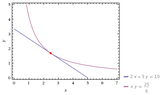
If this company can spend $C(x,y)=10$, which is the greatest quantity that it can produce?We want to maximize $Q(x,y)=xy$ under the condition $2x+3y=10$.
We use the method of Lagrange multipliers. The restriction is $g(x,y)=2x+3y-10=0$.
So we are looking for $\lambda, x ,y$ such that $\nabla Q(x,y)= \lambda \nabla g(x,y)$ and $g(x,y)=0$.
So $y= 2 \lambda, x=3 \lambda \Rightarrow 2x=3y$.
So we get that $x=\frac{10}{4}, y=\frac{5}{3}$.
So the point $\left( \frac{10}{4}, \frac{5}{3}\right)$ is an extremum. How do we deduce that it is maximum?
The production function of a company is $Q(x,y)=xy$. The cost of the production is $C(x,y)=2x+3y$.
If this company can spend $C(x,y)=10$, which is the greatest quantity that it can produce?We want to maximize $Q(x,y)=xy$ under the condition $2x+3y=10$.
We use the method of Lagrange multipliers. The restriction is $g(x,y)=2x+3y-10=0$.
So we are looking for $\lambda, x ,y$ such that $\nabla Q(x,y)= \lambda \nabla g(x,y)$ and $g(x,y)=0$.
So $y= 2 \lambda, x=3 \lambda \Rightarrow 2x=3y$.
So we get that $x=\frac{10}{4}, y=\frac{5}{3}$.
So the point $\left( \frac{10}{4}, \frac{5}{3}\right)$ is an extremum. How do we deduce that it is maximum?
 Alternatively, we can make a drawing from which it will be evident. (Thinking)