Non linear BVP using a shooting algoritm with MATLAB?

[patric44]

Homework Statement

solve the following non linear BVP using shooting method in Matlab ?

Relevant Equations

in the picture

hi guys
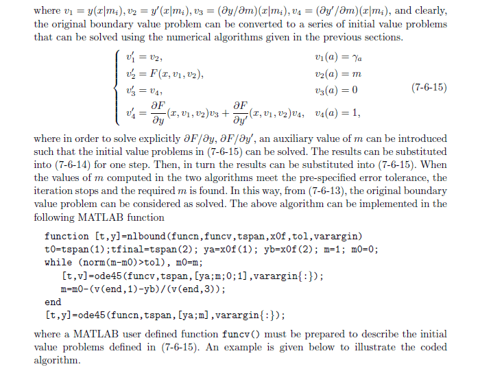
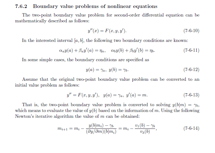
i was trying to use this shooting algorithm from Xue and Chen Scientific Computing with MATLAB book :

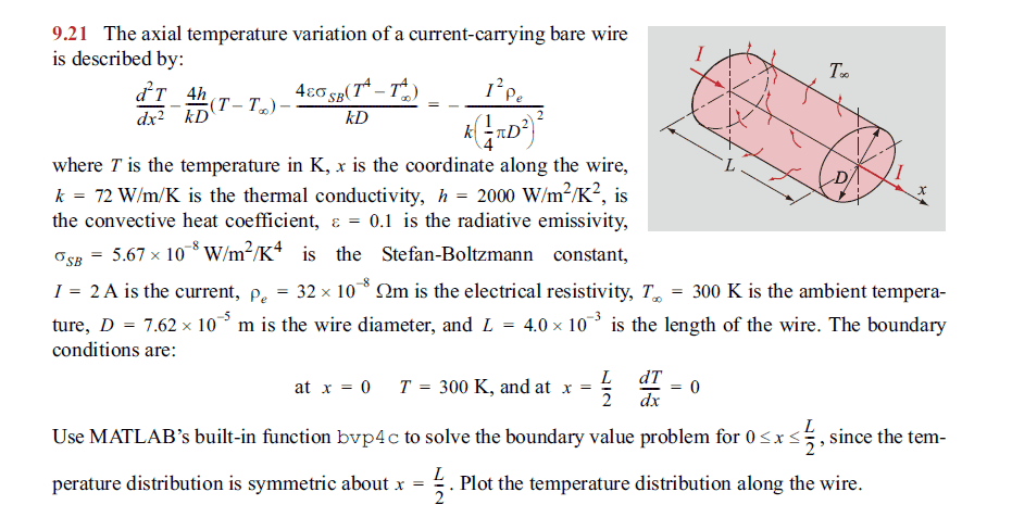
to solve this non linear temperature distribution problem :

i checked my Matlab function multiple times but i am keep getting a nonsense graph for the temperature , can someone cheak what's wrong with my algorithm :

function [t,y] = nlbound(func,funcv,tspan,xof,tol,varargin)
t0 = tspan(1); tf = tspan(2) ; you = xof(1); yb = xof(2);
m=1 ; m0=0;
while(norm(m-m0)>tol), m0=m ;
    [t,v] = ode45(funcv,tspan,[ya;m;0;1],varargin{:});
    m = m0-(v(end,1)-yb)/v(end,3);
end
[t,y] = ode45(func,tspan,[ya;m],varargin{:});
end

the script for the problem :

k = 72;
h = 2000;
epsilon = 0.1;
sigma = 5.67e-8;
i = 2;
rho = 32e-8;
Tinf = 300;
D = 7.62e-5;
L = 4*10^-3;
a1 = (4*h)/(k*D);
a2 = (4*epsilon*sigma)/(k*D);
k = -(i^2*rho)/(k*((pi/4)*D^2)^2);
zeta = k-a1*Tinf-a2*Tinf^4;
% the problem was transformed to a simple form T'' = a1*T+a2*T^4+zeta
f1 = @(t,v)[v(2);a1*v(1)+(a2*v(1)^4)+zeta;v(4);(a1+(4*a2*v(1)^3))*v(3)];
f2 = @(t,x)[x(2);a1*x(1)+a2*x(1)^4+zeta];
x0f = [300,300];
xspan = [0,L];
opts = odeset;
opts.RelTol = 1e-10;
tol = 1e-8;
[t,y] = nlbound(f2,f1,[0,L],[300,300],tol,opts);
plot(t,y(:,1))

i will appreciate any help , thanks

 

[pasmith]

I think the fact that the boundary condition at $x = L/2$ is on $T'$ rather than $T$ may be the problem; the algorithm given is for solving subject to $y(b) = \gamma_b$ rather than $y'(b) = \gamma_b$. So you need to adapt the iteration in (7-6-14) accordingly.

 

[patric44]

i assumed that since the temperature distribution is symmetric about x= L/2 , i would have T(0) = 300 and T(L) = 300 , isn't that right

 

[pasmith]

Does the solution you get satisfy the symmetry constraint?

The only way to enforce that constraint is, as the question suggests. to solve the problem on half of the wire.

You appear to have correctly implemented the algorithm, so if you're not getting the answer you expect then it must be some feature of the particular problem which is to blame. One possibility is that there are multiple solutions to the BVP on the whole rod and you are converging to one which is not the one you expect.

 

[patric44]

Does the solution you get satisfy the symmetry constraint?

The only way to enforce that constraint is, as the question suggests. to solve the problem on half of the wire.

the solution is symmetric ,but as you can see its nonsense :

 

[pasmith]

I implemented this method in Python (using scipy.iintegrate.solve_ivp) and got the same result as you (below left, solid line). However I then solved the problem on the half-rod subject to $T'(L/2) = 0$, and got a more sensible result (below left, dashed line, and below right).

Plotting $T(L|m)$ against $m$ yields the following graph:

From this, we can see that starting the iteration at $m = 1$ is the problem: it puts you to the left of the turning point, and takes you to the wrong solution. Starting with $m \approx 7 \times 10^5$ puts you on the right track. Unfortunately your text's implementation of nlbound doesn't provide a parameter to set an initial guess other than 1.

 

[patric44]

I implemented this method in Python (using scipy.iintegrate.solve_ivp) and got the same result as you (below left, solid line). However I then solved the problem on the half-rod subject to $T'(L/2) = 0$, and got a more sensible result (below left, dashed line, and below right).

View attachment 277141

Plotting $T(L|m)$ against $m$ yields the following graph:

View attachment 277147

From this, we can see that starting the iteration at $m = 1$ is the problem: it puts you to the left of the turning point, and takes you to the wrong solution. Starting with $m \approx 7 \times 10^5$ puts you on the right track. Unfortunately your text's implementation of nlbound doesn't provide a parameter to set an initial guess other than 1.

thank you so much i just tried to change m =1 in the ulbound algorithm to m = 7*10^5 to get me closer to the other solution as you said and it worked

thank you so much you just made my day