KDPhysics
- 73
- 24
I have been trying to numerically solve the Rayleigh-Plesset equation for a sonoluminescing bubble in Python. You can read about this phenomenon here: https://iopscience.iop.org/article/10.1088/0143-0807/34/3/679.
The Rayleigh Plesset equation is a non-linear ODE, which can be solved to find the Radius of a bubble subject to non-linear oscillations due to an external driving sound wave (Sonoluminescence). Here is the form of the equation I used:\begin{equation}\ddot{R} = \frac{1}{R\rho}\Big(P_g-P_0-P(t)-4\mu\frac{\dot{R}}{R}-\frac{2\sigma}{R}+\big(\frac{2\sigma}{R_0}+P_0-P_g\big)\big(\frac{\dot{R}}{R}\big)^{3\kappa}\Big)-\frac{3\dot{R}^2}{2R}\end{equation}
I rewrote this as a system of differential equations (so that ODEINT would process it):
\begin{cases}
\dot{R}=u\\
\dot{u} = \frac{1}{R\rho}\Big(P_g-P_0-P(t)-4\mu\frac{u}{R}-\frac{2\sigma}{R}+\big(\frac{2\sigma}{R_0}+P_0\big)\big(\frac{u}{R}\big)^{3\kappa}\Big)-\frac{3u^2}{2R}
\end{cases}
I used the following parameters and initial conditions:
\begin{cases}R(0) = 2.0\times10^{-6} \text{ m}\\u(0) = 0 \text{ ms}^{-1}\\
\rho = 10^3 \text{ kg m}^3\\
\sigma = 7.25\times10^2 \text{ Nm}^{-1}\\
\mu = 8.9\times10^{-4}\text{ Pa s}\\
P_g = 2330 \text{ Pa}\\
P_0 = 10^5 \text{ Pa}\\
\kappa = 1.33 \end{cases}
The driving pressure from the sound waves is a sine function:
$$P(t)=70000\sin(2\pi(31700t))$$
Here is the python code I have written. It plots both the radius of the bubble and its radial velocity.
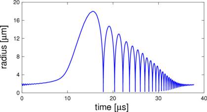
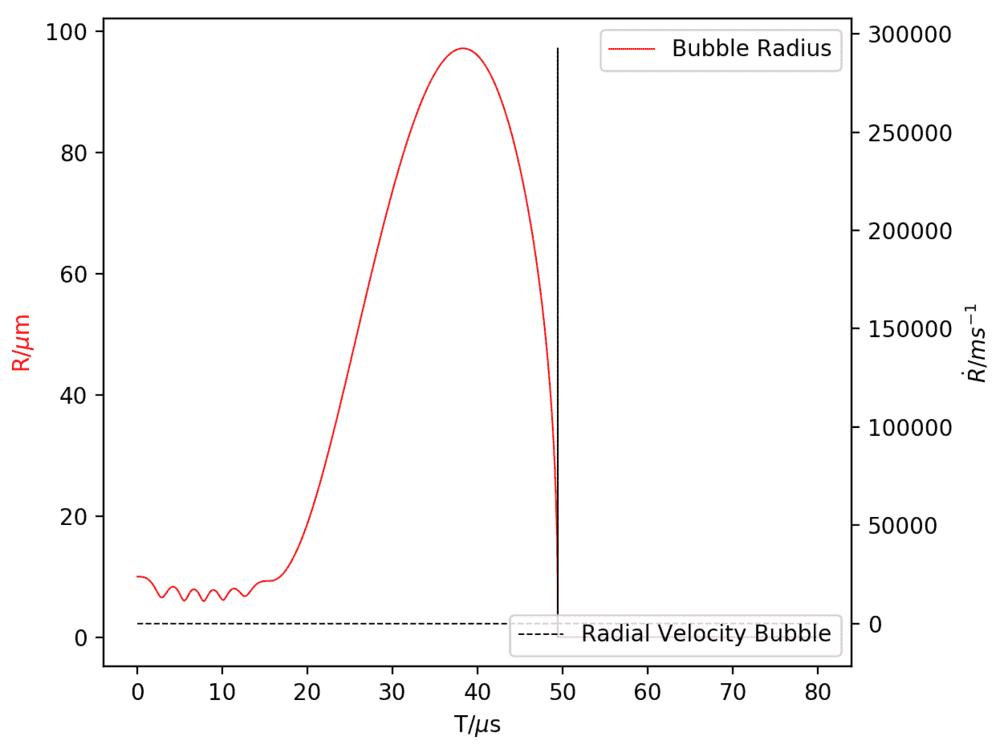
The results from this code however doesn't coincide with literature. Indeed, my code only gives the first collapse, whereas it should show various non-linear oscillations. Not only, the velocity plot shows that the bubble expands at supersonic speeds (which also doesn't coincide with literature given the present parameters).
Here is what the output should look like:
Here is what the code gives:
Please CompSci geniuses help me ...
EDIT: here is the stack exchange thread I created regarding the same question. Hopefully, someone will answer on one of the two forums.
The Rayleigh Plesset equation is a non-linear ODE, which can be solved to find the Radius of a bubble subject to non-linear oscillations due to an external driving sound wave (Sonoluminescence). Here is the form of the equation I used:\begin{equation}\ddot{R} = \frac{1}{R\rho}\Big(P_g-P_0-P(t)-4\mu\frac{\dot{R}}{R}-\frac{2\sigma}{R}+\big(\frac{2\sigma}{R_0}+P_0-P_g\big)\big(\frac{\dot{R}}{R}\big)^{3\kappa}\Big)-\frac{3\dot{R}^2}{2R}\end{equation}
I rewrote this as a system of differential equations (so that ODEINT would process it):
\begin{cases}
\dot{R}=u\\
\dot{u} = \frac{1}{R\rho}\Big(P_g-P_0-P(t)-4\mu\frac{u}{R}-\frac{2\sigma}{R}+\big(\frac{2\sigma}{R_0}+P_0\big)\big(\frac{u}{R}\big)^{3\kappa}\Big)-\frac{3u^2}{2R}
\end{cases}
I used the following parameters and initial conditions:
\begin{cases}R(0) = 2.0\times10^{-6} \text{ m}\\u(0) = 0 \text{ ms}^{-1}\\
\rho = 10^3 \text{ kg m}^3\\
\sigma = 7.25\times10^2 \text{ Nm}^{-1}\\
\mu = 8.9\times10^{-4}\text{ Pa s}\\
P_g = 2330 \text{ Pa}\\
P_0 = 10^5 \text{ Pa}\\
\kappa = 1.33 \end{cases}
The driving pressure from the sound waves is a sine function:
$$P(t)=70000\sin(2\pi(31700t))$$
Here is the python code I have written. It plots both the radius of the bubble and its radial velocity.
Python:
import numpy as np
from matplotlib import pyplot as plt
from scipy.integrate import odeint

# define equations
def equation(y0, t):
    R, u = y0
    return u, (P_g-P_0-70000*np.sin(2*np.pi*31700*t)-2*sigma/R-4*miu*u/R+(2*sigma/R_0+P_0-P_g)*(R_0/R)**(3*k))/(R*rho)-3*u**2/(2*R)

# initial conditions
R_0 = 0.00001
u_0 = 0

# parameters
rho = 1000
sigma = 0.0728
miu = 8.9*10**(-4)
P_g = 2330
P_0 = 10000
k = 1.33

time = np.arange(0, 0.00008, 0.00000000025)R_1 = odeint(equation, [R_0, u_0], time)

V = R_1[:,1]
R = R_1[:,0]*10**6
mtimes = time*10**6

#plot results

fig, ax1 = plt.subplots()

ax1.set_xlabel("T/$\mu$s")
ax1.set_ylabel("R/$\mu$m", color = "red")
ax1.plot(mtimes, R, linewidth = 0.7, label = "Bubble Radius", color = "red")

ax2 = ax1.twinx()  # instantiate a second axes that shares the same x-axis

ax2.set_ylabel("$\dot{R}$/$ms^{-1}$")  # we already handled the x-label with ax1
ax2.plot(mtimes, V, linestyle = "dashed", color = "black", linewidth = 0.7, label = "Radial Velocity Bubble")
ax1.legend()
ax2.legend(loc = "lower right")

fig.tight_layout()  # otherwise the right y-label is slightly clipped
plt.show()
The results from this code however doesn't coincide with literature. Indeed, my code only gives the first collapse, whereas it should show various non-linear oscillations. Not only, the velocity plot shows that the bubble expands at supersonic speeds (which also doesn't coincide with literature given the present parameters).
Here is what the output should look like:
Here is what the code gives:
Please CompSci geniuses help me ...
EDIT: here is the stack exchange thread I created regarding the same question. Hopefully, someone will answer on one of the two forums.
Last edited:
