Orbit of the Earth - numerical methods leapfrog

Click For Summary
SUMMARY

The discussion focuses on implementing the LeapFrog numerical method to simulate the Earth's orbit and calculate kinetic and potential energy. The user modified the function to include gravitational forces and energy calculations but encountered an overflow error. Key equations include the gravitational force dz[2]=-G*M*m/r and the kinetic energy calculation E_kin = 0.5*m*(vx**2+vy**2). The results show that total energy remains relatively constant, with minor oscillations attributed to the LeapFrog method.

PREREQUISITES
  • Understanding of Newtonian mechanics and gravitational forces
  • Familiarity with Python programming and libraries such as NumPy and Matplotlib
  • Knowledge of numerical integration techniques, specifically the LeapFrog method
  • Basic concepts of kinetic and potential energy calculations
NEXT STEPS
  • Explore advanced numerical integration techniques beyond LeapFrog, such as Runge-Kutta methods
  • Learn about energy conservation in orbital mechanics and its implications
  • Investigate the effects of varying mass and distance on gravitational interactions
  • Study the implementation of error analysis in numerical simulations
USEFUL FOR

Students and professionals in physics, computational science, and engineering who are interested in orbital mechanics and numerical simulations of dynamical systems.

Graham87
Messages
72
Reaction score
16
Homework Statement
Plot gravitational potential energy and kinetic energy
Relevant Equations
-GMm/r, 0.5mv^2
I am attempting this homework exercise part b).
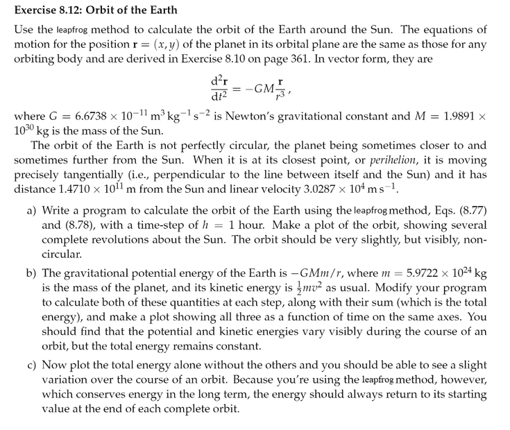
1.png

I've modified my code but I get error overflow message. My goal is to modify my code so it returns kinetic and potential energy of Earth's orbit.
I made a new f(z,t) and modified the rows 99 and 100 with dz[2]=-G*M*m/r, and dz[3]=0.5*m*y**2 but obviously it didn't work.

Python:
import matplotlib.pyplot as plt
import numpy as np
import scipy.integrate as spi

G = 6.6738*10**-11
M = 1.9891*10**30
h = 3600
y = 1.4710*10**11
vx = 3.0287*10**4

def LeapFrog(f, t_start, t_stop, z0, h):

    t_vec = np.arange(t_start, t_stop, h)
    n = len(t_vec)
    d = len(z0)
    z_vec = np.zeros((n, d))
    z_vec[0,:] = z0
    z_half_step=z_vec[0 , :] + (1/2)*h*f(z0,t_vec[0])
   
   
    for i in range(0, n - 1):
        z_vec[i+1,:]=z_vec[i,:] + h*f(z_half_step, t_vec[i])
        z_half_step += h*f(z_vec[i+1,:], t_vec[i])      return t_vec, z_vec,def f(z,t):   #dz/dt
   
    x=z[0]
    y=z[1]
    vx=z[2]
    vy=z[3]
    r=np.sqrt(x**2+y**2)

    dz=np.zeros(4)
   
    dz[0]=vx
    dz[1]=vy
    dz[2]=-G*M*x/r**3
    dz[3]=-G*M*y/r**3

    return dz

t_start = 0
t_stop = 24*365*h*5 #5 years
z0 = np.array([0,y,vx,0])
t_vec, z_vec = LeapFrog(f, t_start, t_stop, z0, h)
figure, ax = plt.subplots()

plt.title("Orbit of the Earth")
plt.plot(0,0,'yo', label = 'Sun positon')
plt.plot(z_vec[:,0],z_vec[:,1], 'g', markersize=1, label='Earth trajectory')
ax.set_aspect('equal')

ax.set(xlim=(-1.55*10**11, 1.55*10**11), ylim = (-1.55*10**11, 1.55*10**11))
a_circle = plt.Circle((0, 0), 1.4710*10**11, fill=False,color='r')
ax.add_artist(a_circle)
ax.set_aspect('equal')

legend = plt.legend(['Sun position','Earths 5-year trajectory','Perfect circle'],loc='center left', bbox_to_anchor=(1, 0.5))

plt.show()
"""

We can see that the trajectory of the Earth for 5 years is very slightly non-circular.

"""

"""b"""

m = 5.9722*10**24
def f(z,t):   #dz/dt
   
    x=z[0]
    y=z[1]
    vx=z[2]
    vy=z[3]
    r=np.sqrt(x**2+y**2)

    dz=np.zeros(4)
   
    dz[0]=vx
    dz[1]=vy
    dz[2]=-G*M*m/r
    dz[3]=0.5*m*y**2

    return dz

t_start = 0
t_stop = 24*365*h*5 #5 years
z0 = np.array([0,y,vx,0])
LeapFrog(f, t_start, t_stop, z0, h)
 
Last edited:
Physics news on Phys.org
The equation of motion is exactly the same as in part (a) so you don't need to change the integration. What information do you think you need to calculate kinetic and potential energy?
 
  • Like
Likes   Reactions: Graham87
pbuk said:
The equation of motion is exactly the same as in part (a) so you don't need to change the integration. What information do you think you need to calculate kinetic and potential energy?
Aha! So I use the result from part a) to compute the energies:

Python:
x,y,vx,vy = z_vec.T
r=np.sqrt(x**2+y**2)
E_kin = 0.5*m*(vx**2+vy**2)
E_pot = -G*M*m/r
E = E_kin+E_pot

plt.title('Energies function of time')
plt.plot(t_vec,E_pot)
plt.plot(t_vec,E_kin)
plt.plot(t_vec,E)
plt.legend(['Potential energy','Kinetic energy', 'Total energy'])
plt.show()

plt.title('Total E(t)')
plt.plot(t_vec,E)
plt.show()

I get these plots now. Did I plot it correctly? Shouldn't total energy oscillate between 0?

2.png
 
Last edited:
  • Like
Likes   Reactions: pbuk
Graham87 said:
I get these plots now. Did I plot it correctly?
Looks about right: the key point is that total energy is more or less constant, (with a relatively small oscillation which is an artefact of the leapfrog method: you'll probably cover this in the next lecture).
 
  • Love
Likes   Reactions: Graham87

Similar threads

  • · Replies 6 ·
Replies
6
Views
2K
  • · Replies 4 ·
Replies
4
Views
2K
  • · Replies 12 ·
Replies
12
Views
2K
  • · Replies 5 ·
Replies
5
Views
3K
  • · Replies 7 ·
Replies
7
Views
3K
  • · Replies 2 ·
Replies
2
Views
4K
  • · Replies 4 ·
Replies
4
Views
3K
Replies
3
Views
1K
  • · Replies 7 ·
Replies
7
Views
3K
  • · Replies 6 ·
Replies
6
Views
2K