Plotting the trajectory of a particle in polar coordinates

[Lambda96]

Homework Statement

Plot the curve of $\rho(t)=\rho_0 + \rho_1 \sin^2(4 \pi t)$

Relevant Equations

none

Hi,

Unfortunately, I am not quite sure whether I have solved/plotted the following task correctly

I started by resolving the expression $\phi=2 \pi t$ to t so that I can represent $\rho(t)$ with $\rho(\phi)$

The vector $\vec{e}_r$ was written in my lecture as follows $\vec{e}_{\rho}$ , $\vec{e}_{\rho}= \left(\begin{array}{c} \cos(\phi) \\ \sin(\phi) \end{array}\right)$

Then the position vector is $\vec{r}(\phi)=\rho(\phi) \vec{e}_{\rho}=(\rho_0+\rho_1 \sin^2(2 \phi) ) \left(\begin{array}{c} \cos(\phi) \\ \sin(\phi) \end{array}\right)$

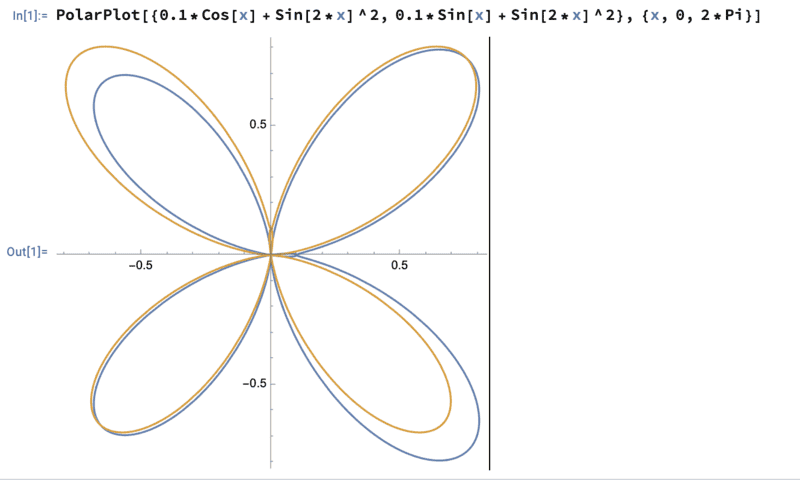
Then I plotted this expression using Mathematica from $0$ to $2 \pi$

Is that correct? Because doesn't the two different colors mean that I got the trajectory for two different particles instead of just one?

 

[TSny]

Note that the expression $\rho = 0.1 + \sin^2(4\pi t)$ is always greater than or equal to 0.1. So, the trajectory never gets closer than 0.1 to the origin.

The format for Mathematica's PolarPlot is

Here, $r$ is just your $\rho$ expressed as a function of $\phi$, but without the $\vec{e}_{\rho}= \left(\begin{array}{c} \cos(\phi) \\ \sin(\phi) \end{array}\right)$. By putting in $\vec{e}_{\rho}= \left(\begin{array}{c} \cos(\phi) \\ \sin(\phi) \end{array}\right)$, you are essentially going to Cartesian coordinates where the x and y components are expressed in terms of the parameter $\phi$. In that case, you could use Mathematica's ParametricPlot. However, I think using PolarPlot is simpler here.

 

[Steve4Physics]

In addition to what @TSny said, can I add this.

Then the position vector is $\vec{r}(\phi)=\rho(\phi) \vec{e}_{\rho}=(\rho_0+\rho_1 \sin^2(2 \phi) ) \left(\begin{array}{c} \cos(\phi) \\ \sin(\phi) \end{array}\right)$

Note that $(\rho_0+\rho_1 \sin^2(2 \phi))$ is a scalar quantity. So

$(\rho_0+\rho_1 \sin^2(2 \phi) )\left(\begin{array}{c} \cos(\phi) \\ \sin(\phi) \end{array}\right)$

is equal to

$\left(\begin{array}{c} \rho_0\cos(\phi)+\rho_1 \sin^2(2 \phi)\cos(\phi) \\ \rho_0\sin(\phi)+\rho_1 \sin^2(2 \phi)\sin(\phi) \end{array}\right)$

This doesn't match what you entered in Mathematica.

You might want practise/check by plotting a few simple curves of known shapes.

 

[Lambda96]

Thank you TSny and Steve4Physics for your help

I have now redone the plot and got the following:

 

[TSny]

Looks good.

 

[TSny]

If you want to use the command ParametricPlot, then the format is

So, for this problem we would have

Or, maybe less confusing,

 

[Lambda96]

Thank you TSny for your help and also thank you for showing me how to plot the curve with ParametricPlot Since Mathematica is relatively new to me, this helped me a lot.