Questions about Taylor dispersion in laminar pipeflow

[tjuaachen]

In the equation characterizing the mass transfer in laminar flow, the radial variation of velocity and concentration can be lumped into the axial dispersion term as below:

After reading the original paper about Taylor dispersion, I know how to derive this equation. But I am still not able to understand it intuitively. How can the dispersion term make such a great difference here? Why bother ourselves with using the mean concentration rather than the concentration of single point? I hope my puzzle can be dispelled here and I will appreciate any replies.

 

[Chestermiller]

In the equation characterizing the mass transfer in laminar flow, the radial variation of velocity and concentration can be lumped into the axial dispersion term as below:
View attachment 210475
View attachment 210476
After reading the original paper about Taylor dispersion, I know how to derive this equation. But I am still not able to understand it intuitively.

After seeing the derivation, are you able to articulate the fundamental physical mechanism involved here?

How can the dispersion term make such a great difference here?

Why don't you put some typical numbers into the equation and see how the Taylor diffusivity compares with the molecular diffusivity.

Why bother ourselves with using the mean concentration rather than the concentration of single point? I hope my puzzle can be dispelled here and I will appreciate any replies.

You use the mean concentration rather than the concentrations at single points because it's much easier to analyze as a 1D problem than a 2D problem. For typical situations, analytic solutions are even available. Plus, you are often only interested in the average concentration. Plus, if the fluid comes out into some kind of collection vessel, the concentration variations are mixed away anyway.

 

[tjuaachen]

After seeing the derivation, are you able to articulate the fundamental physical mechanism involved here?

Why don't you put some typical numbers into the equation and see how the Taylor diffusivity compares with the molecular diffusivity.

You use the mean concentration rather than the concentrations at single points because it's much easier to analyze as a 1D problem than a 2D problem. For typical situations, analytic solutions are even available. Plus, you are often only interested in the average concentration. Plus, if the fluid comes out into some kind of collection vessel, the concentration variations are mixed away anyway.

Dr Chet, A huge thank for your detailed and inspiring reply. In my opinion, within the infinitesimal control volume (2*pi*r dr*dz), the convection and radial molecular diffusion occur. But when the equation derived from this control volume is transformed into the average form, I am confused about the physical meaning of the derivative dispersion term, though I can accept it in terms of math.

If the concentration is not the area averaged, I can still imagine the physical process in my mind. But when it is area averaged, things get complicated since t's hard to do the calculus in our brain.

 

[Chestermiller]

Dr Chet, A huge thank for your detailed and inspiring reply. In my opinion, within the infinitesimal control volume (2*pi*r dr*dz), the convection and radial molecular diffusion occur. But when the equation derived from this control volume is transformed into the average form, I am confused about the physical meaning of the derivative dispersion term.

The parabolic velocity profile causes the concentrations near the center of the tube to travel axially faster than the concentrations near the wall. So this creates radial concentration variations, which result in radial diffusion. The combination of radially varying axial convection by the parabolic profile plus radial diffusion translates into the equivalent of axial diffusion, based on the mean concentration. This is my understanding of the basic mechanism.

This same type of dispersion also occurs in groundwater systems involving transport of contaminant species in subsurface geological formations. The permeability of the sediments in the layers varies with depth within the formation and, for horizontal flows of aqueous contaminant laden fluid, there is an equivalent dispersion in the direction of flow.

 

[tjuaachen]

The parabolic velocity profile causes the concentrations near the center of the tube to travel axially faster than the concentrations near the wall. So this creates radial concentration variations, which result in radial diffusion. The combination of radially varying axial convection by the parabolic profile plus radial diffusion translates into the equivalent of axial diffusion, based on the mean concentration. This is my understanding of the basic mechanism.

Thank you for the sharing. But is it a coincidence to discover this translation? or in other words, are there some physical or mathematical clues implying this translation?

 

[tjuaachen]

How did Sir Geoffrey Taylor figure out this method?

 

[Chestermiller]

Thank you for the sharing. But is it a coincidence to discover this translation? or in other words, are there some physical or mathematical clues implying this translation?

Are you asking how G. I. Taylor came to the realization that his could be modeled as axial dispersion? I think he realized it from analysis experimental data on concentration vs time for the discharge stream from a pipe. Once he saw that the concentration vs time was close to the same as that which would be obtained from axial dispersion, he was motivated to do the mathematical analysis of the problem.

Incidentally, one of the thrills of my lifetime was meeting G. I. Taylor in person at the 150th anniversary of the University of Michigan in 1967. Now, in 2017, the University of Michigan is having its 200th anniversary. I was particularly thrilled because my PhD thesis was on the Taylor stability of viscoelastic Couette flow.

 

[tjuaachen]

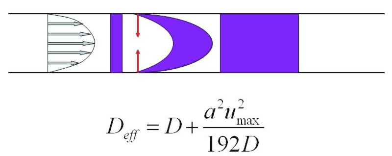
Are you asking how G. I. Taylor came to the realization that his could be modeled as axial dispersion? I think he realized it from analysis experimental data on concentration vs time for the discharge stream from a pipe. Once he saw that the concentration vs time was close to the same as that which would be obtained from axial dispersion, he was motivated to do the mathematical analysis of the problem.

Incidentally, one of the thrills of my lifetime was meeting G. I. Taylor in person at the 150th anniversary of the University of Michigan in 1967. Now, in 2017, the University of Michigan is having its 200th anniversary. I was particularly thrilled because my PhD thesis was on the Taylor stability of viscoelastic Couette flow.

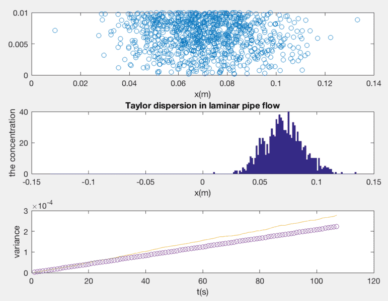
Dr Chet, after several hours' effort, it is the final result of my simulation as above. Though, up to now, I acquaint myself thoroughly with the Taylor dispersion, its physical mechanism still make no sense to me. I even doubt if the Taylor dispersion is really existent. Or perhaps, it is just created by Taylor for the convenience. Is it reasonable to think so? Is it a sound point?

Here is the Matlab code. You can implement in one button if you like.
%taylor dispersion. Let's go!

clear all

clc

N=1000;

b=0.01;

u0=0.01;

x=zeros(1000,1);

y=b*rand(1000,1);

D=10^-5;

dt=0.1;
for NT=1:10000 ,

y=y+(2*D*dt)^0.5*randn(N,1);%random walk in the y direction

for n=1:1000

if(y(n)<0)

y(n)=abs(b);

else if(y(n)>b)

y(n)=2*b-y(n);

end

end

end

up=4*u0*(y/b).*(1-y/b);

x=x+(2*D*dt)^0.5*randn(N,1)+up*dt;%random walk+convection

%y=y+(2*D*dt)^0.5*randn(N,1);

xedge=[-max(x):max(x)/100:max(x)];

variancex(NT)=var(x);

taylor(NT)=0.01^2*0.01^2/(192*D)*NT*dt*4;

subplot(3,1,2)
numx=histc(x,xedge);

%figure

%hold on

bar(xedge,numx,'histc')%draw the bar plot to approximate the area averaged concentration

xlabel('x(m)')

ylabel('the concentration')

title('Taylor dispersion in laminar pipe flow')

subplot(3,1,1)
plot(x,y,'o')

xlabel('x(m)')

ylabel('y(m)')

subplot(3,1,3)
plot(variancex)

xlabel('t(s)')

ylabel('variance')

hold on

plot(taylor,'o')%compare the taylor diffusivity with the calculated number

pause(0.01);

end

 

[Chestermiller]

I don't understand what you did. I thought you were solving the 2D convection/diffusion equation for parabolic flow in a pipe, and then calculating the mixing cup average concentration as a function of position at a given time, or at a function of time at a given position.

 

[tjuaachen]

I don't understand what you did. I thought you were solving the 2D convection/diffusion equation for parabolic flow in a pipe, and then calculating the mixing cup average concentration as a function of position at a given time, or at a function of time at a given position.

Absolutely, Dr Chet. It's exactly what I have done. I count the numbers located in a specific narrow range, which ,I think, corresponds to the area averaged concentration. And the final result turns out that the variance agree well with the value calculated from the Taylor dispersion diffusivity.

Anyway, let's come back to the physical process. What I want to know is "is the Taylor dispersion really existent?"or "is it just an imaginary process created on the basis of mathematical derivation?"

 

[Chestermiller]

Absolutely, Dr Chet. It's exactly what I have done. I count the numbers located in a specific narrow range, which ,I think, corresponds to the area averaged concentration. And the final result turns out that the variance agree well with the value calculated from the Taylor dispersion diffusivity.

Anyway, let's come back to the physical process. What I want to know is "is the Taylor dispersion really existent?"or "is it just an imaginary process created on the basis of mathematical derivation?"

It depends on how you want to apply the result. If you need to know the detailed radial variations in concentration, then it won't give you that. If you want to follow the mixing cup average concentration profiles that develop axially along the pipe, or the time variation of the mixing cup average at the exit of the pipe, then it's a valuable tool. And, if you are dealing with a chemical reactor in which laminar flow is occurring, it provides an accurate approximation for including the effect of axial dispersion.

 

[tjuaachen]

It depends on how you want to apply the result. If you need to know the detailed radial variations in concentration, then it won't give you that. If you want to follow the mixing cup average concentration profiles that develop axially along the pipe, or the time variation of the mixing cup average at the exit of the pipe, then it's a valuable tool. And, if you are dealing with a chemical reactor in which laminar flow is occurring, it provides an accurate approximation for including the effect of axial dispersion.

Your patience is highly appreciated. Let's be crystal clear. Is the Taylor dispersion a concrete physical process? Or it's just a hypothetical process created by Sir Taylor for the sake of convenience and interest. Please answer my question directly, Doctor Chet.

 

[Chestermiller]

Your patience is highly appreciated. Let's be crystal clear. Is the Taylor dispersion a concrete physical process? Or it's just a hypothetical process created by Sir Taylor for the sake of convenience and interest. Please answer my question directly, Doctor Chet.

I think that we are dealing with semantics here. Taylor dispersion is an very accurate mathematical approximation to the exact solution of trace species transport encountered in a system involving flow with a velocity profile in one direction and diffusion perpendicular to that direction. When we talk about Taylor dispersion, we engineers and scientists all know what we mean. The concept has broad applicability way beyond just laminar flow transport in a tube. Its main area of applicability is in trace species transport in flow through porous media and packed beds. We don't want to have to calculate the detailed concentration profiles of the trace species within each and every one of the pores of the bed on a scale of the pore diameter. Even if we knew the exact interstitial geometry, the calculation would be incredibly time consuming, for no reason. We would like to determine the concentration variations on a much larger scale, knowing only the superficial fluid velocity from Darcy's law.

In a porous medium or packed bed, the flow channels are very non-uniform, and flow along some streamlines is very high velocity, while flow along other streamlines is very slow. This is analogous to the situation in Sir Geoffrey's single tube. So we know that Taylor dispersion is going to be a feature of the trace species transport present in a porous medium or packed bed. All we need to do to carry out calculations on such a system is to perform an experiment in which we measure the dispersivity of core samples in the laboratory. Then we can use the superficial velocity calculated for the flow in the actual porous bed in conjunction with the laboratory measured value of the dispersivity to accurately model the species transport in bed.

I don't know whether this answers your questions, but it is the best I can do.