Analyzing Motion: Deriving Displacement Graphs from First Principles

AI Thread Summary
The discussion focuses on deriving displacement graphs from first principles, starting with initial conditions where displacement is h above the ground and gravity acts negatively. The initial displacement equation is derived using integration, resulting in a parabolic shape for the first portion of the graph. The challenge arises in the second interval, where the user struggles to derive the correct s(t) function due to the discontinuity at the bounce. Suggestions include using a spring model to smooth the curve and adjusting integration limits to account for cyclic motion. The conversation emphasizes the need for clarity in defining integration variables and limits to achieve the desired displacement function.
Old_sm0key
Messages
17
Reaction score
0
Homework Statement
Not a homework question per se. I revisited introductory kinematics, as taught at British A Level, and am struggling to reproduce the stadnard plots for displacement and velocity versus time.
Relevant Equations
The standard 1D kinematics equations plus introductory differentiation
Initial displacement is h above the ground ie ##s\left ( t =0\right )=h##. I've chosen the ground as the vertical origin with upwards as the positive direction. Gravity will therefore always act in negative direction throughout. Here are the graphs I which to reproduce from first principles, where the motion starts at the red vertical line owing to my initial conditions:
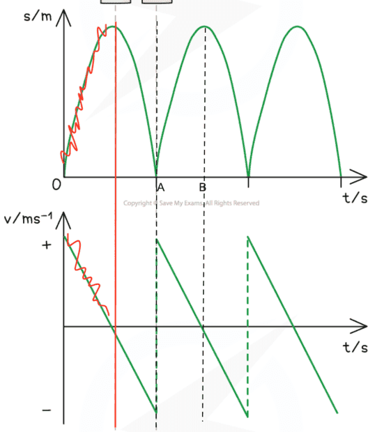
kinematics.png


##0\leqslant t< A##
Starting from ##v=u+at## we derive displacement thus:
$$\int_{0}^{t} vdt^\prime=\int_{0}^{t}\left ( u+at \right )dt^\prime$$
$$s\left ( t \right )-h=ut+\frac{1}{2}at^2$$
Using conditions ##t=0,u=0, a=-g\, \forall t \to s\left ( t \right )=h-\frac{1}{2}gt^2## which would give a parabola for first portion of displacement graph. So happy.
The corresponding velocity graph is ##\frac{\mathrm{d} s}{\mathrm{d} t}=-gt##, so giving a negative straight line. Happy.

##A\leqslant t< B##
Now I'm stuck with the displacement curve because I cannot exploit ##t=0## on the integral limits to simplify the maths...?
Plus it seems a fudge to suddenly invoke ##s\left ( t \right )=vt-\frac{1}{2}at^2## that I see in some textbooks.
 
Physics news on Phys.org
If you want to avoid the fudge of the discontinuity of the velocity at the bounce, you can model the ball as having a spring attached to its bottom. This will round off the curve with a sinusoidal and give it a collision duration of half a period. You can sharpen it by increasing the spring constant ##k.## so that the period of oscillations is much much smaller than the time between bounces.
 
With what are you trying to reproduce them? If in a spreadsheet, it's just a matter of first converting t to be in the range 0 to A using MOD.
 
Thanks both, however I probs didn't make myself too clear.

(I accept the velocity discontinuity @ bounce ie precluding differentiation)

I want to derive the s vs t equation, just like I did above, now for ##A\leqslant t< B## to produce the shape shown in plot. Just can't get the right s(t) function..!
 
Old_sm0key said:
$$\int_{0}^{t} vdt^\prime=\int_{0}^{t}\left ( u+at \right )dt^\prime$$
In order to correctly distinguish between your integration variable and the limits, this should be$$\int_{0}^{t} vdt^\prime=\int_{0}^{t}\left ( u+at^\prime \right )dt^\prime$$If I’ve understood what you are asking…

Let T be the duration of each ‘cycle’ (from t=0 to A). This is a constant you can express in terms of h and g.

You have chosen to make B halfway through the 2nd cycle. Not sure if that’s deliberate, but no matter.

You can use the method you used for the 1st cycle - but change the integration limits: from T to t+T/2. Because the process is cyclic, your initial conditions at the start of each cycle are identical to those at t=0.
 
Old_sm0key said:
Thanks both, however I probs didn't make myself too clear.

(I accept the velocity discontinuity @ bounce ie precluding differentiation)

I want to derive the s vs t equation, just like I did above, now for ##A\leqslant t< B## to produce the shape shown in plot. Just can't get the right s(t) function..!
Why not include B in the interval? I.e. ##\ A\le t \le B \ ##
You can actually go father, to the next zero of ##s(t)##, maybe call it ##C##.

At ##t=B## you have ##s(t) = h## and ##v(t) = 0##.

Either use indefinite integrals and evaluate the constants of integration according to the above values (at ##t=B## ) ,

or use definite integrals and integrate from ##t## to ##B##, or from ##B## to ##t##. Just be consistent with the direction of the integration.
 
Old_sm0key said:
derive the s vs t equation
In post #1 you said you wanted to plot the function, and I gave you a way to do that in post #3. Now you say "derive" it, but in what sense do that? From a differential equation, or as an integral?

Or are you just looking to write the function s(t)? Depends what functions you accept as valid in it. There will have to be one which is not continuously differentiable. As I mentioned, there is mod(), which is not only used in spreadsheets.
https://en.wikipedia.org/wiki/Modulo_operation
 
Back
Top