Best fit to an oscillating function

Click For Summary

Discussion Overview

The discussion revolves around finding an appropriate mathematical function to fit a numerically obtained oscillating function that exhibits both high-frequency oscillations and a lower-frequency envelope. Participants explore various approaches, including Fourier transforms and signal processing techniques, to refine the fit to the observed data.

Discussion Character

  • Exploratory
  • Technical explanation
  • Mathematical reasoning

Main Points Raised

  • The original poster (OP) presents a function and seeks advice on how to improve its fit to a plotted oscillating function with high-frequency oscillations and a lower-frequency envelope.
  • Some participants suggest using a Fourier transform of the original signal to express it as a sum of sines and cosines.
  • There is a discussion about potential numerical issues with the Fourier transform due to the high frequency of oscillations within low-frequency cycles.
  • One participant proposes downshifting the signal to make it more amenable to Fourier analysis by adjusting the carrier frequency.
  • Another participant mentions the need for an imaginary unit "i" in the exponential function used for downshifting the frequency.
  • There is a suggestion to sample the data less frequently to simplify the analysis, potentially taking every 10th or 100th sample.
  • A participant shares an attempt to use Mathematica to analyze the edges of the OP's plot and questions whether the desired low-frequency signal could be derived from the average of the upper and lower boundaries of the outlines.

Areas of Agreement / Disagreement

Participants express various approaches to the problem, but there is no consensus on a single method or solution. Multiple competing views and techniques remain under discussion.

Contextual Notes

Participants note potential limitations related to numerical issues in Fourier transforms and the complexity of downshifting the signal, which may require further elaboration.

kelly0303
Messages
573
Reaction score
33
Hello! I have a plot of a function, obtained numerically, that looks like the red curve in the attached figure. It is hard to tell, but if you zoom in enough, inside the red shaded area you actually have oscillations at a very high frequency, ##\omega_0##. On top of that you have some sort of envelope, with a lower frequency, ##\omega_1##. I am trying to find a function that comes as close as possible to this. In green is what I obtained using:

$$A\sin(\omega_1 t/2)^2(1+\cos(\omega_0t/2))^2$$
where ##A## is just an overall amplitude (and I shifted everything for clarity). However I am not sure how to get the rest of the behaviour, basically fill in the gaps in my function relative to the red one. Can someone advice me on what functional form would I need to add to my expression to get that? Thank you!
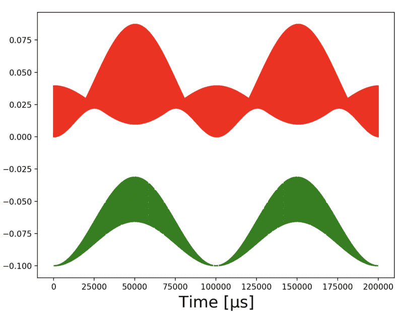
func.png
 
Physics news on Phys.org
Have you considered a Fourier transform?
 
  • Like
Likes   Reactions: Scottpm, berkeman, FactChecker and 1 other person
DaveE said:
Have you considered a Fourier transform?
Thank you! What exactly do you mean? Fourier transform of what?
 
kelly0303 said:
Thank you! What exactly do you mean? Fourier transform of what?
Fourier transform of your original signal. It will tell you how to write it as a sum of sines and cosines. If you absolutely to have it as an envelope times a constant oscillation, it will take a bit more work.

If you don't mind sharing the data (at least privately), I would like to take a go at it.
 
DrClaude said:
Fourier transform of your original signal. It will tell you how to write it as a sum of sines and cosines. If you absolutely to have it as an envelope times a constant oscillation, it will take a bit more work.

If you don't mind sharing the data (at least privately), I would like to take a go at it.
Ah I see, thank you I will look into that. There is no actual data. The red-line is generated by numerically integrating on ODE, but I am attaching below the points used in that plot.
 

Attachments

If each low-frequency cycle contains thousands (or even hundreds) of high frequency cycles, you may have numerical problems with the Fourier transform. You will have to process way more samples than are really needed to answer your question.

Instead, shift the signal down so that your ##\omega_0 ## is lower, keeping your ##\omega_1## structure the same. (Then when you plot it, you will be able to see, let's say 20 cycles of ##\omega_0 /2## within one cycle of ##\omega_1##. After this down shift the signal will be more amenable to Fourier transform with a moderate number of samples.

You can down shift the "carrier" frequency by multiplying the original signal by ##e^{-\omega_2 t}## where ##\omega_2## is a few percent less than ##\omega_0##.

Edit:
As hutchpd has said, you need an 'i' in the exponential.

Downshifting will be a bit more complicated than I have indicated above... I will post later with more details, or maybe someone can fill in the details.
 
Last edited:
You need an "i" in the exponential yes?
 
hutchphd said:
You need an "i" in the exponential yes?
Yup.

Edit: Wait, I believe there was an i in the original... But anyway.
 
  • Like
Likes   Reactions: hutchphd
It will probably work if you just take every 10th or 100th sample (leaving you with say 20 samples per "big" cycle) and pretend that's your actual signal.
 
  • #10
Just for fun, I asked Mathematica to find the edges in the OP's plot:

1678151257093.png


I am now trying to find out if Mathematica can convert the bitmap edges to vectors. Any ideas?

Also, is it correct that the desired low freq. signal is the average of the upper and lower boundaries of the outlines above?
 

Similar threads

  • · Replies 17 ·
Replies
17
Views
3K
  • · Replies 1 ·
Replies
1
Views
3K
Replies
9
Views
2K
Replies
3
Views
1K
  • · Replies 2 ·
Replies
2
Views
1K
  • · Replies 1 ·
Replies
1
Views
2K
  • · Replies 4 ·
Replies
4
Views
2K
  • · Replies 2 ·
Replies
2
Views
2K
Replies
8
Views
2K
Replies
7
Views
1K