Calculus of variations on odd dimensional manifolds

[mma]

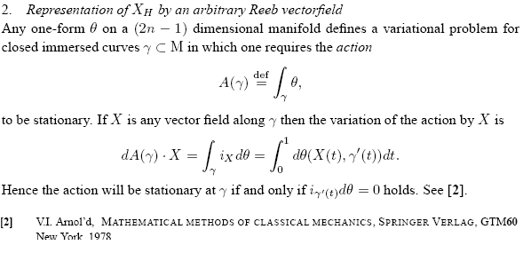
I saw a nice formulation of the variation on odd dimensional manifolds in the paper of http://arxiv.org/abs/math-ph/0401046" :

The referenced book of Arnold uses completely different formalism than this.
I don't see clearly the connection between the traditional calculus of variations and this formulas (for example, where are the boundary conditions here ? Why only closed curves are considered?). Could somebody offer a book or other resource that uses the same formalism for the calculus of variations?

 

[mma]

Sorry, I gave a false link.

The proper lik is http://www.google.hu/url?sa=t&sourc...7yMCw&usg=AFQjCNGhVxdr6Z8yvVEw_RTm3_ZbamPCzA"

 

[mma]

I'd like to prove that

$$\int_\gamma{\iota_Xd\theta}=\left.{\frac{dA(\gamma_t)}{dt}}\right |_{t=0}$$​

where $$\gamma_t$$ is a curve flowed by $$t$$ in the flow generated by $$X$$, that is,

$$\gamma_t(\tau) = \Phi_X(\gamma(\tau),t)$$​

where $$\Phi_X: M\times \mathbb{R} \to M$$ is the flow generated by the vector field $$X$$, that is $$t \mapsto \Phi(p,t)$$ is the integrel curve of $$X$$ passing through the point $$p\in M$$.

But I have no idea how to prove this.

Any hint would be appreciated.

 

[mma]

In an $$\{x_1,x_2,...,x_n\}$$ coordinate chart,the LHS is:

$$\int_\gamma{\iota_Xd\theta}= \int_0^1 d\theta(X(\gamma(\tau)),\gamma'(\tau))d\tau =\int_0^1 \sum_{i,j}\frac{\partial\theta_j}{\partial x_i}(X_i(\gamma(\tau))\gamma'_j(\tau)-X_j(\gamma(\tau))\gamma'_i(\tau)) d\tau$$​

,the RHS is:

$$\left.\frac{d}{dt}\right |_{t=0}\int_{\gamma(t)}\theta =\int_0^1\sum_i\left.\frac{d}{dt}\right |_{t=0}\theta_i(\Phi(\gamma(\tau),t)\gamma'_i(\tau) d\tau$$​

Why are they equal?

 

[mma]

I'd like to prove that

$$\int_\gamma{\iota_Xd\theta}=\left.{\frac{dA(\gamma_t)}{dt}}\right |_{t=0}$$​

where $$\gamma_t$$ is a curve flowed by $$t$$ in the flow generated by $$X$$, that is,

$$\gamma_t(\tau) = \Phi_X(\gamma(\tau),t)$$​

where $$\Phi_X: M\times \mathbb{R} \to M$$ is the flow generated by the vector field $$X$$, that is $$t \mapsto \Phi(p,t)$$ is the integrel curve of $$X$$ passing through the point $$p\in M$$.

The proof seems quite simple if we consider only open curves (i.e. having $$\gamma(0) \neq \gamma(1)$$) and require that $$X(\gamma(0))=X(\gamma(1))=0$$.

In this case, according Stokes' theorem,

$$A(\gamma_t) - A(\gamma) = \int_{\gamma_t}\theta - \int_{\gamma}\theta=\oint_{\gamma_t-\gamma}\theta = \int_{S_t}d\theta$$​

,where $$S_t$$ is a 2-dimensional surface streched on $$\gamma_t-\gamma$$, in other words, having boundary $$\partial S_t = \gamma_t-\gamma$$.

On $$S_t$$ we can introduce a coordinate chart

$$(\xi,\eta) \mapsto \Phi_X(\gamma(\xi),\eta) = \gamma_\eta(\xi)$$​

,hence

$$\int_{S_t}d\theta=\int_0^t\int_0^1 \, d\theta(\gamma_\eta '(\xi),X(\gamma_\eta(\xi))\, d\xi\,d\eta$$​

,so

$$\left.{\frac{dA(\gamma_t)}{dt}}\right |_{t=0} =\left.\frac{d}{dt}\right |_{t=0}\int_{S_t}d\theta=\int_0^1 \, d\theta(\gamma '(\xi),X(\gamma(\xi))\, d\xi=\int_\gamma{\iota_Xd\theta}$$
​

Am I right?