SUMMARY
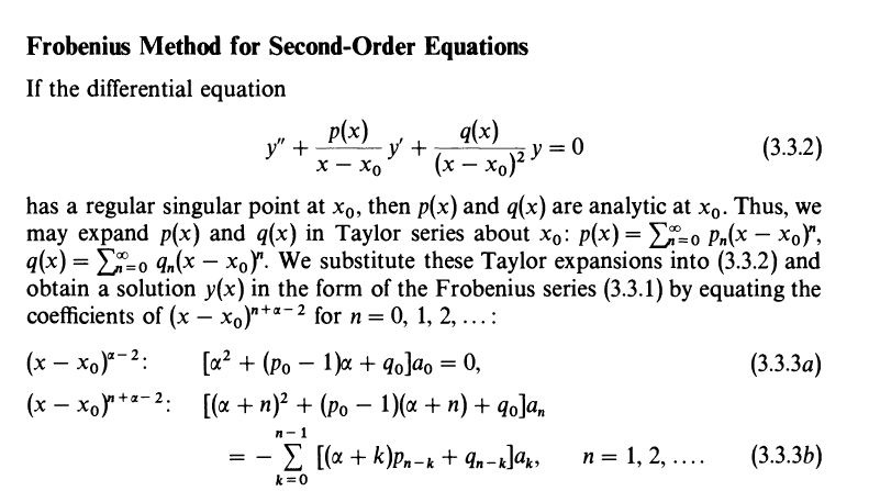
The discussion centers on the derivation of the indicial exponent in the Frobenius method, specifically referencing Equation 3.3.3b from the book "Asymptotic Methods and Perturbation Theory." The solution involves expressing y(x) as A(x)*(x-x0)^α, where A(x) is expanded using a Taylor series. The participants analyze the series multiplication technique, emphasizing the importance of correctly applying the Cauchy product to derive the coefficients of the resulting power series.
PREREQUISITES
- Understanding of the Frobenius method for solving differential equations
- Familiarity with Taylor series expansions
- Knowledge of power series and their convergence
- Basic grasp of asymptotic analysis techniques
NEXT STEPS
- Study the Frobenius method in detail, focusing on its application to linear differential equations
- Learn about the Cauchy product of series and its implications in power series multiplication
- Explore the concept of indicial roots and their significance in differential equations
- Investigate the role of asymptotic methods in perturbation theory
USEFUL FOR
Mathematicians, physicists, and engineers involved in solving differential equations, particularly those utilizing the Frobenius method and asymptotic analysis techniques.
