Discussion Overview
The discussion revolves around the concept of destination points in harmonic sequences, specifically exploring whether a destination point can be reached for any value of θ in the range 0 ≤ θ < 2𝜋. Participants also inquire about the existence of a function that encompasses all destination points.
Discussion Character
- Exploratory
- Technical explanation
- Mathematical reasoning
Main Points Raised
- Some participants propose that the harmonic sequence will continue for all values of θ and question if a destination point will be reached.
- One participant asserts that for 0 < θ < 2𝜋, the path will converge to a limit point, which can be expressed using complex numbers and a series summation.
- A detailed mathematical expression for the limit point is provided, involving a series and logarithmic functions, with a specific case noted for θ = π.
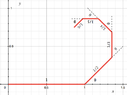
- Another participant shares a graphical representation of the limit points based on the provided formula, indicating specific coordinates for certain values of θ.
- There is mention of the Leibniz series and its relation to the limit points for θ = π/2, with calculations presented for the corresponding x and y values.
Areas of Agreement / Disagreement
Participants express varying viewpoints on the existence and nature of destination points, with some agreeing on the convergence of the series while others raise questions about the complexity of finding a function that represents the set of destination points. The discussion remains unresolved regarding the broader implications of these findings.
Contextual Notes
Limitations include the dependence on the definitions of convergence and the specific conditions under which the series is evaluated. The mathematical steps leading to the limit point are not fully resolved, and the complexity of finding a function that represents all destination points is acknowledged.