Science Advisor
Gold Member
- 1,404
- 1,668
- TL;DR
- Using a cloud chamber in a quantum 2-slit experiment gives linear tracks of uniform length that overwhelmingly point back to halfway between the slits (but with a very few outliers) and a track density that exhibits the familiar interference pattern.
The Motivation
Spurred by some interesting back and forth with @PeterDonis in a recent forum thread, I present here my attempt to answer the titular question. I begin with the Schrödinger equation for the wave function ##\psi## of a free charged particle of mass ##m##:$$i\hbar\frac{\partial\psi}{\partial t}=-\frac{\hbar^{2}}{2m}\nabla^{2}\psi\tag{1}$$and define the probability density ##\rho## and the probability-current/flux density ##\vec{J}## in the usual ways:$$\rho\equiv\psi^{\ast}\psi\, ,\;\vec{J}\equiv-\frac{i\hbar}{2m}\left(\psi^{\ast}\nabla\psi-\psi\nabla\psi^{\ast}\right)=\frac{\hbar}{m}\text{Im}\left(\psi^{\ast}\nabla\psi\right)\tag{2a,b}$$The scalar density ##\rho## is of course responsible for the familiar interference-pattern on the target screen of the standard 2-slit configuration. But if that target is switched to a cloud chamber, vector information is required to predict the directions of the tracks therein, and that information resides in ##\vec{J}##. Recall that the differential cross section for single quantum scattering is defined in terms of probability fluxes to be ##d\sigma\left(\theta,\phi\right)/d\Omega=r^{2}\Vert\vec{J}_{\text{scat}}\Vert/\Vert\vec{J}_{\text{in}}\Vert## where ##\vec{J_{\text{in}}}## is the incident flux (see, e.g., Ballentine, Quantum Mechanics: A Modern Development, §16.1). Two common examples of incident fluxes are (proportional to): 1) ##\left(\hbar k/m\right)\hat{z}\,## for an incoming particle-beam plane wave that impacts a target in an accelerator experiment and 2) ##\left(\hbar k/mr^{2}\right)\hat{r}## gives the outgoing spherical wave centered on an alpha-emitter in the Mott analysis of cloud chamber tracks. But these two examples are in no way exhaustive: any ##\vec{J}##-field can serve as an incident flux, including that arising from a 2-slit interferometer bombarding a cloud chamber. As first demonstrated by Mott, if the incident charged particle is sufficiently energetic and interacts only weakly and inelastically with the vapor molecules in the chamber, the resulting ##d\sigma/d\Omega## will be sharply peaked in the forward direction ##\vec{J}_{\text{in}}/\Vert\vec{J}_{\text{in}}\Vert## at the first scattering and then again at each subsequent scattering, until the particle energy is expended, leaving behind a linear trail of ionized vapor having a characteristic length (see Multiple scattering of charged particles by N atoms, §V). Since this "stopping-distance" is governed by the particle's incoming energy, a monoenergetic flux of such particles yields a spatial-distribution of tracks with identical lengths.
Explaining the tracks in a 2-slit interferometer/cloud-chamber system is therefore grounded in the following three principles:
With this preamble out of the way, it's time to "just shut up and calculate" the flux ##\vec{J}\,## incident on a cloud chamber from 2 slits. Given the following (idealized) configuration:
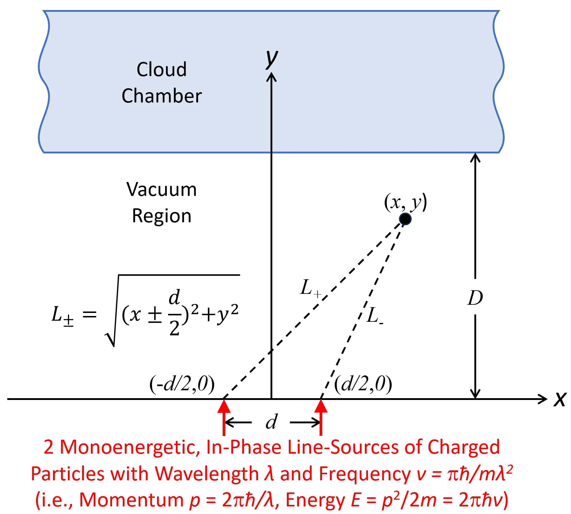
the physical solution of eq.(1) is expressed in terms of the Hankel function ##H_{0}^{\left(1\right)}##:$$\psi\left(x,y,t\right)=Ne^{-2\pi i\nu t}\left(H_{0}^{\left(1\right)}\left(2\pi L_{+}/\lambda\right)+H_{0}^{\left(1\right)}\left(2\pi L_{-}/\lambda\right)\right)\tag{3}$$where ##N## is an arbitrary normalization constant. This solution is singled out because the two terms in (3) embody the required outgoing cylindrical waves, each propagating away from the ##z##-directed line-sources located at ##\left(\mp d/2,0\right)##, that ultimately impinge on the cloud chamber. (I use line-sources to avoid the inessential complication of finite slit-widths.) Since ##N## is arbitrary, I choose it to set the normalized wave function ##\psi_N## to unity "on-axis" at the entrance to the chamber; i.e., ##\psi_N\left(0,D\right)=1##. I can also drop the time-harmonic term ##e^{-2\pi i\nu t}## since it disappears from ##\rho## and ##\vec{J}##. Here is the resulting wave function:$$\psi_{N}\left(x,y\right)=\frac{H_{0}^{\left(1\right)}\left(\pi\sqrt{\left(d+2x\right)^{2}+4y^{2}}/\lambda\right)+H_{0}^{\left(1\right)}\left(\pi\sqrt{\left(d-2x\right)^{2}+4y^{2}}/\lambda\right)}{2H_{0}^{\left(1\right)}\left(\pi\sqrt{d^{2}+4D^{2}}/\lambda\right)}\tag{4}$$along with its gradient:$$\begin{align}&\nabla\psi_{N}\left(x,y\right) =\nonumber \\ & -\frac{\pi}{\lambda}\left(\frac{\left(d+2x\right)H_{1}^{\left(1\right)}\left(\pi\sqrt{\left(d+2x\right)^{2}+4y^{2}}/\lambda\right)}{H_{0}^{\left(1\right)}\left(\pi\sqrt{d^{2}+4D^{2}}/\lambda\right)\sqrt{\left(d+2x\right)^{2}+4y^{2}}}-\frac{\left(d-2x\right)H_{1}^{\left(1\right)}\left(\pi\sqrt{\left(d-2x\right)^{2}+4y^{2}}/\lambda\right)}{H_{0}^{\left(1\right)}\left(\pi\sqrt{d^{2}+4D^{2}}/\lambda\right)\sqrt{\left(d-2x\right)^{2}+4y^{2}}}\right)\hat{x} \nonumber \\ & -\frac{2\pi}{\lambda}\left(\frac{y\,H_{1}^{\left(1\right)}\left(\pi\sqrt{\left(d+2x\right)^{2}+4y^{2}}/\lambda\right)}{H_{0}^{\left(1\right)}\left(\pi\sqrt{d^{2}+4D^{2}}/\lambda\right)\sqrt{\left(d+2x\right)^{2}+4y^{2}}}+\frac{y\,H_{1}^{\left(1\right)}\left(\pi\sqrt{\left(d-2x\right)^{2}+4y^{2}}/\lambda\right)}{H_{0}^{\left(1\right)}\left(\pi\sqrt{d^{2}+4D^{2}}/\lambda\right)\sqrt{\left(d-2x\right)^{2}+4y^{2}}}\right)\hat{y} \nonumber \tag{5}\end{align}$$Equations (4) and (5) are the ingredients I add to (2a,b) to create the density fields ##\rho\left(x,y\right),\vec{J}\left(x,y\right)##, but I won't burden the reader by explicitly displaying their cumbersome analytical forms. It suffices to simply let my Mathematica software deal with the algebra and focus on visualizing the results.
To illustrate, I select the parameters ##d=5\lambda,D=40\lambda## and define the dimensionless relative-flux ##\vec{J}_{R}\left(x,y\right)\equiv\vec{J}\left(x,y\right)/\Vert\vec{J}\left(0,40\lambda\right)\Vert##, calculate the probability density and flux values, and then plot those in a few different ways.
The Probability and Flux Densities
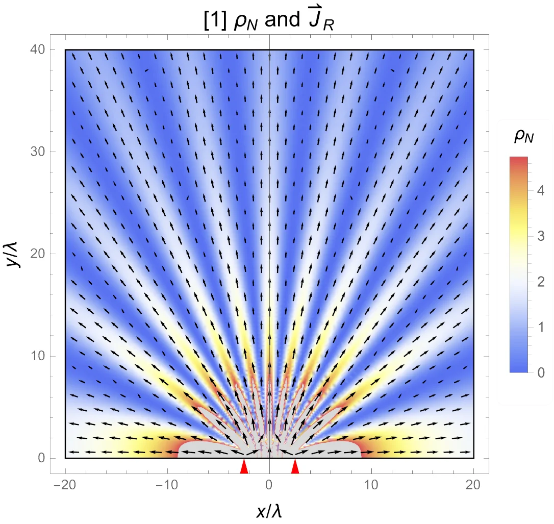
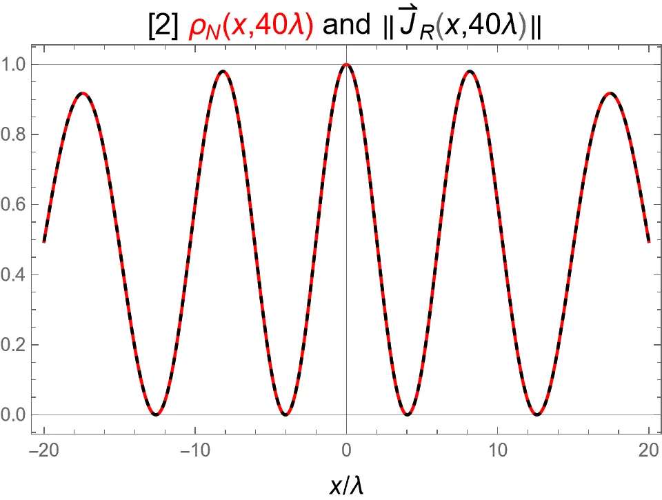
Plot [1] clearly exhibits the interference bands in ##\rho_N## characteristic of the 2-slit configuration, as well as the size and direction of the outflowing probability-flux vectors ##\vec{J_R}##. Note that those vectors (mostly) follow the interference bands and are longer at the blue-white peaks and shorter near the pure-blue valleys of ##\rho_N##. Indeed, plot [2] shows the distributions of ##\rho_N## and ##\Vert\vec{J_R}\Vert## to be virtually identical at the entrance to the cloud chamber, where they differ at most by a few parts in ##10^{-4}##, implying that the track-density in the chamber displays the same band structure as the spot-density on the target of the standard 2-slit experiment.
The Flux Direction
Beyond the "near-field" region in plot [1], the flux vectors primarily follow flow lines that more or less point back toward the origin, half-way between the slits. But on close inspection, it's also evident that a few short vectors in the nulls of ##\rho_N## are clearly non-parallel to the overall flow direction; moreover, some of the flow lines apparently "swerve" through a null before resuming their original direction. To investigate this "non-radial" behavior, I use the unit-vector ##\hat{r}\equiv\left(x\hat{x}+y\hat{y}\right)/\sqrt{x^{2}+y^{2}}## to decompose the total flux vector into radial (r) and non-radial (nr) components:$$\vec{J}_{R\left(\text{r}\right)}=\left(\hat{r}\cdot\vec{J}_{R}\right)\hat{r}\;,\quad\vec{J}_{R\left(\text{nr}\right)}=\vec{J}_{R}-\left(\hat{r}\cdot\vec{J}_{R}\right)\hat{r}\tag{6a,b}$$from which it follows that the magnitude of the non-radial flux density at any point is:$$\Vert\vec{J}_{R\left(\text{nr}\right)}\left(x,y\right)\Vert=\Vert\vec{J}_{R}\left(x,y\right)\Vert\sqrt{1-\left(\hat{r}\left(x,y\right)\cdot\hat{J}_{R}\left(x,y\right)\right)^{2}}\tag{7}$$and the angle of deviation of the non-radial flux density from the radial "boresight" direction is:$$\delta_{\left(\text{nr}\right)}\left(x,y\right)=\cos^{-1}\left(\hat{r}\left(x,y\right)\cdot\hat{J}_{R}\left(x,y\right)\right)\tag{8}$$Below are plots of these two quantities evaluated at the entrance to the cloud chamber:
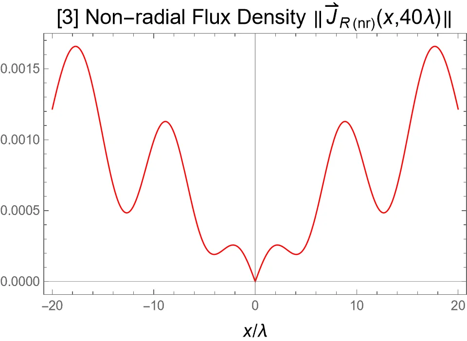
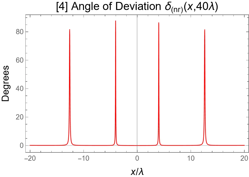
Observe in plot [3] that the non-radial flux density is everywhere merely a tiny fraction of the total flux density. This minuteness is reflected in the expectation value of the total non-radial flux:$$\left\langle \Vert\vec{J}_{R\left(\text{nr}\right)}\Vert\right\rangle =\frac{\intop_{-20\lambda}^{20\lambda}dx\,\Vert\vec{J}_{R}\left(x,40\lambda\right)\Vert\sqrt{1-\left(\hat{r}\left(x,40\lambda\right)\cdot\hat{J}_{R}\left(x,40\lambda\right)\right)^{2}}}{\intop_{-20\lambda}^{20\lambda}dx\,\Vert\vec{J}_{R}\left(x,40\lambda\right)\Vert}=0.00151\approx\frac{1}{661}\tag{9}$$So out of every ##661## chamber tracks, all but ##1## are expected to point directly back to the center between the slits. And just how misaligned is that one exceptional track apt to be? Per plot [4], the deviation angle ##\delta_\text{(nr)}## can be as high as ##87°##, but that's only in narrow bands at the minima of ##\rho_N## where the probability of finding the particle is very low. Elsewhere, the deviation is essentially zero. In fact, the overall expected value of the deviation is just:$$\left\langle \delta_{\left(\text{nr}\right)}\right\rangle =\frac{\intop_{-20\lambda}^{20\lambda}dx\,\Vert\vec{J}_{R}\left(x,40\lambda\right)\Vert\cos^{-1}\left(\hat{r}\left(x,40\lambda\right)\cdot\hat{J}_{R}\left(x,40\lambda\right)\right)}{\intop_{-20\lambda}^{20\lambda}dx\,\Vert\vec{J}_{R}\left(x,40\lambda\right)\Vert}=0.0869°\tag{10}$$ Non-radial tracks are therefore fairly rare and most often only very-slightly misaligned. But that's not to say that tracks with larger deviations don't occur with lower probabilities. For example, the probability ##P\left(\delta_{\left(\text{nr}\right)}\geq5{^\circ}\right)## is ##2.78\times 10^{-5}##; i.e., the observed deviation angle equals or exceeds ##5{^\circ}## about once in every ##36,000## tracks.
The Flux Streamlines
A more refined view of the current flow is available by plotting the streamlines (integral curves) of the ##\vec{J_R}##-vector field:
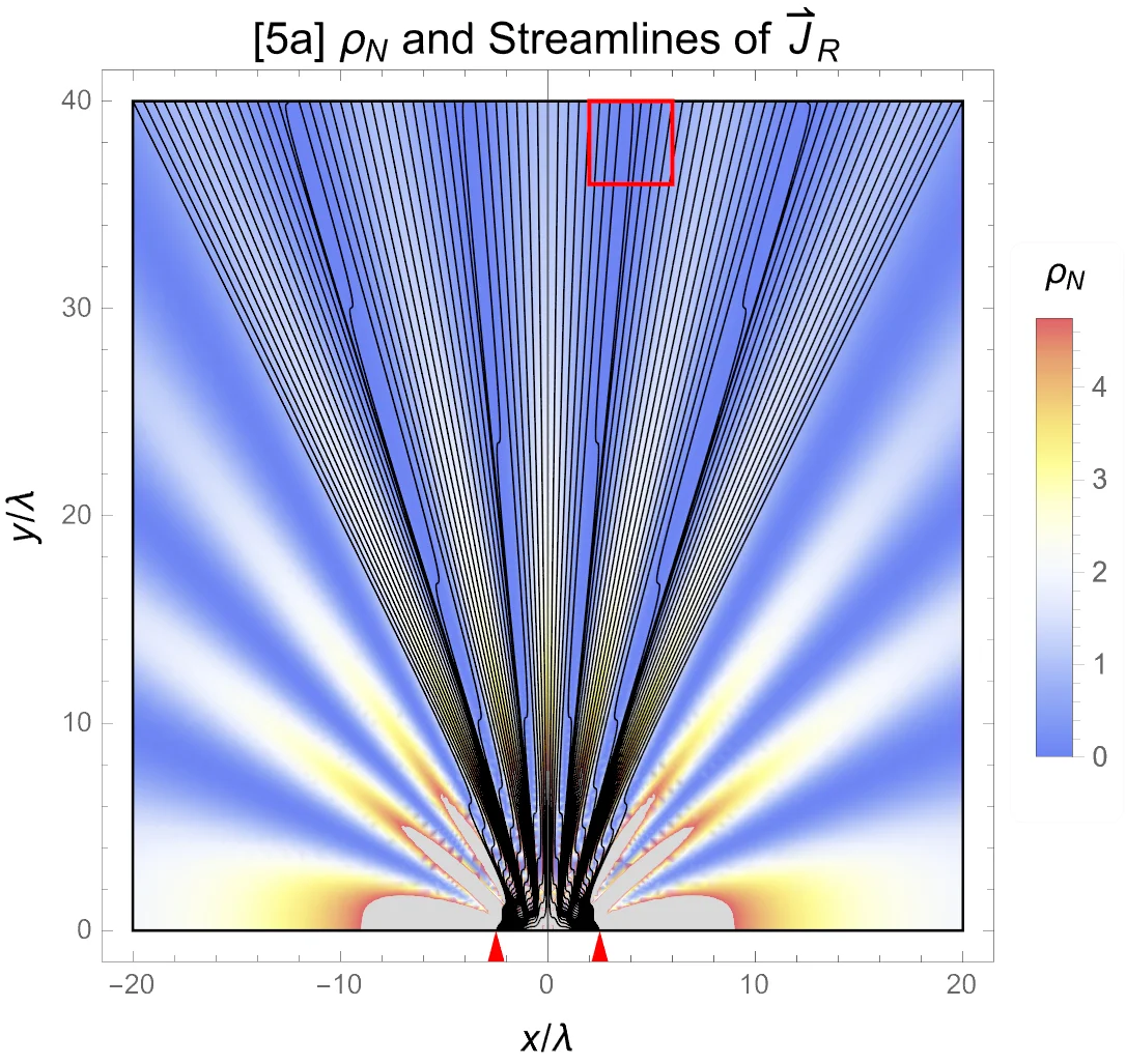
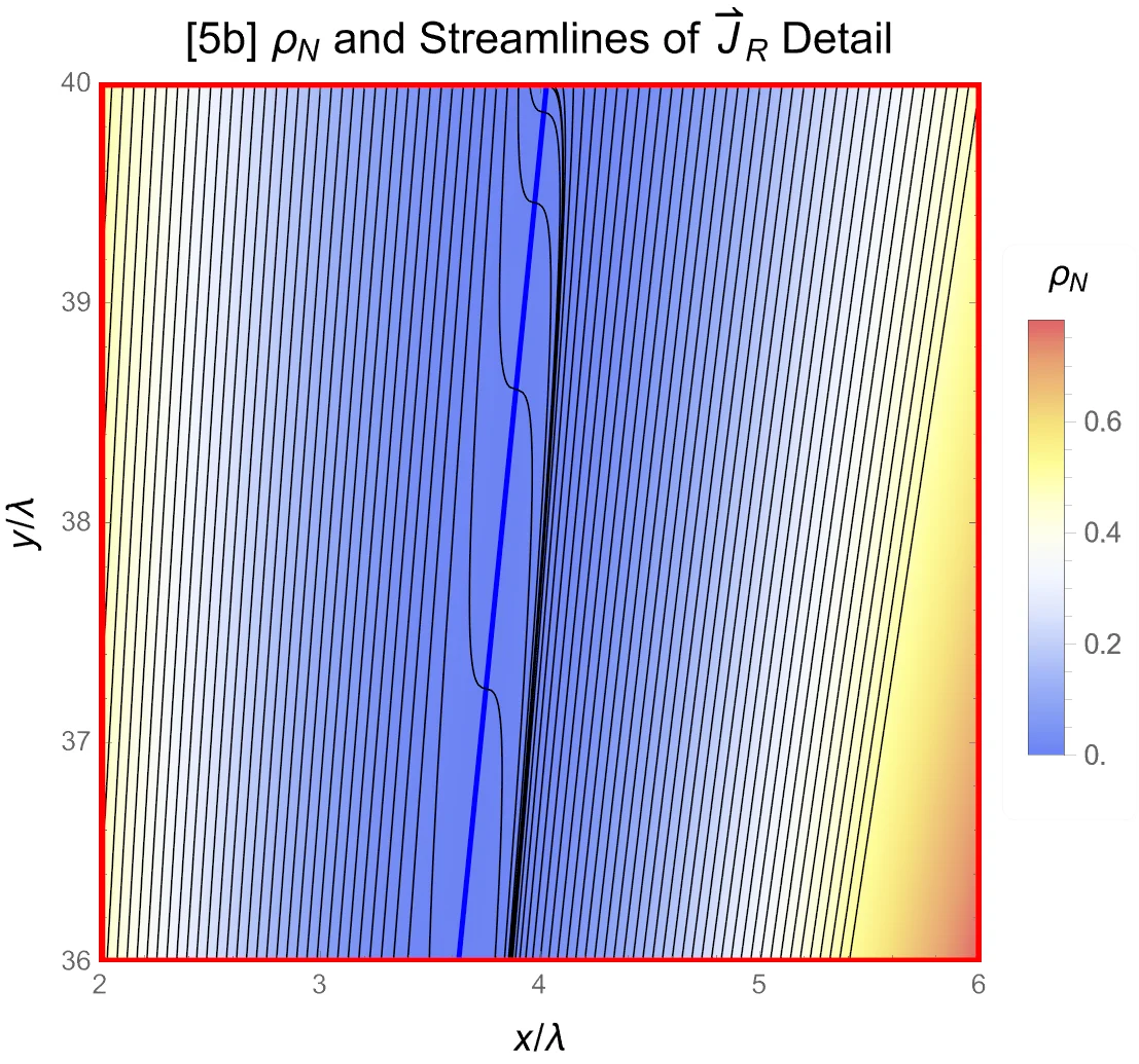
It's evident in [5a] that the current streamlines bend as they pass near to and cross through a null "valley" of the probability density ##\rho_N##, and then resume their radial path on the opposite side of that valley. This is especially clear in the magnified view [5b] where I explicitly demark the minimum of ##\rho_N## by the deep-blue line. I conclude that the direction of the streamline tangent-vector ##\hat{J}_R## swings dramatically during these crossing transitions, and whenever such a swing occurs near the entrance to the cloud chamber, the resulting track will be non-radial.
(Historical aside: Images akin to plot [5a] are often seen in discussions of Bohm's pilot-wave interpretation of quantum mechanics (https://en.wikipedia.org/wiki/De_Broglie–Bohm_theory) wherein the streamlines of current flux are understood to be the actual trajectories of the particles as they travel away from their source, toward and then into the cloud chamber.)
The Wrap-Up
Below is a schematic representation of the cloud chamber tracks, their bands of varying density, and the locations from which they appear to originate:
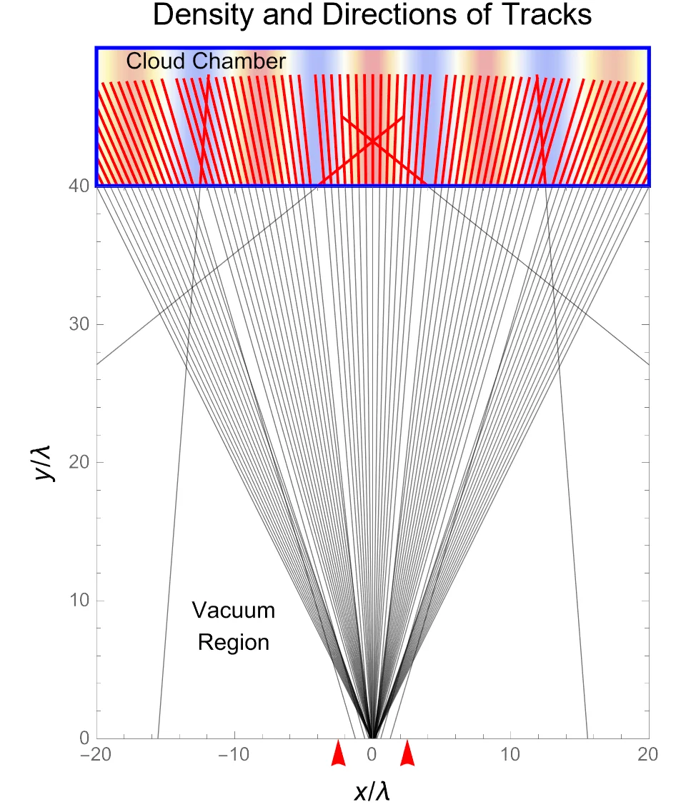
I draw these final conclusions:

Spurred by some interesting back and forth with @PeterDonis in a recent forum thread, I present here my attempt to answer the titular question. I begin with the Schrödinger equation for the wave function ##\psi## of a free charged particle of mass ##m##:$$i\hbar\frac{\partial\psi}{\partial t}=-\frac{\hbar^{2}}{2m}\nabla^{2}\psi\tag{1}$$and define the probability density ##\rho## and the probability-current/flux density ##\vec{J}## in the usual ways:$$\rho\equiv\psi^{\ast}\psi\, ,\;\vec{J}\equiv-\frac{i\hbar}{2m}\left(\psi^{\ast}\nabla\psi-\psi\nabla\psi^{\ast}\right)=\frac{\hbar}{m}\text{Im}\left(\psi^{\ast}\nabla\psi\right)\tag{2a,b}$$The scalar density ##\rho## is of course responsible for the familiar interference-pattern on the target screen of the standard 2-slit configuration. But if that target is switched to a cloud chamber, vector information is required to predict the directions of the tracks therein, and that information resides in ##\vec{J}##. Recall that the differential cross section for single quantum scattering is defined in terms of probability fluxes to be ##d\sigma\left(\theta,\phi\right)/d\Omega=r^{2}\Vert\vec{J}_{\text{scat}}\Vert/\Vert\vec{J}_{\text{in}}\Vert## where ##\vec{J_{\text{in}}}## is the incident flux (see, e.g., Ballentine, Quantum Mechanics: A Modern Development, §16.1). Two common examples of incident fluxes are (proportional to): 1) ##\left(\hbar k/m\right)\hat{z}\,## for an incoming particle-beam plane wave that impacts a target in an accelerator experiment and 2) ##\left(\hbar k/mr^{2}\right)\hat{r}## gives the outgoing spherical wave centered on an alpha-emitter in the Mott analysis of cloud chamber tracks. But these two examples are in no way exhaustive: any ##\vec{J}##-field can serve as an incident flux, including that arising from a 2-slit interferometer bombarding a cloud chamber. As first demonstrated by Mott, if the incident charged particle is sufficiently energetic and interacts only weakly and inelastically with the vapor molecules in the chamber, the resulting ##d\sigma/d\Omega## will be sharply peaked in the forward direction ##\vec{J}_{\text{in}}/\Vert\vec{J}_{\text{in}}\Vert## at the first scattering and then again at each subsequent scattering, until the particle energy is expended, leaving behind a linear trail of ionized vapor having a characteristic length (see Multiple scattering of charged particles by N atoms, §V). Since this "stopping-distance" is governed by the particle's incoming energy, a monoenergetic flux of such particles yields a spatial-distribution of tracks with identical lengths.
Explaining the tracks in a 2-slit interferometer/cloud-chamber system is therefore grounded in the following three principles:
- The density of tracks is proportional to ##\Vert\vec{J}_{\text{in}}\Vert##.
- The direction of tracks is given by the unit-vector ##\hat{J}_{\text{in}}\equiv\vec{J}_{\text{in}}/\Vert\vec{J}_{\text{in}}\Vert##.
- The lengths of tracks are all identical for a monoenergetic flux.
With this preamble out of the way, it's time to "just shut up and calculate" the flux ##\vec{J}\,## incident on a cloud chamber from 2 slits. Given the following (idealized) configuration:
the physical solution of eq.(1) is expressed in terms of the Hankel function ##H_{0}^{\left(1\right)}##:$$\psi\left(x,y,t\right)=Ne^{-2\pi i\nu t}\left(H_{0}^{\left(1\right)}\left(2\pi L_{+}/\lambda\right)+H_{0}^{\left(1\right)}\left(2\pi L_{-}/\lambda\right)\right)\tag{3}$$where ##N## is an arbitrary normalization constant. This solution is singled out because the two terms in (3) embody the required outgoing cylindrical waves, each propagating away from the ##z##-directed line-sources located at ##\left(\mp d/2,0\right)##, that ultimately impinge on the cloud chamber. (I use line-sources to avoid the inessential complication of finite slit-widths.) Since ##N## is arbitrary, I choose it to set the normalized wave function ##\psi_N## to unity "on-axis" at the entrance to the chamber; i.e., ##\psi_N\left(0,D\right)=1##. I can also drop the time-harmonic term ##e^{-2\pi i\nu t}## since it disappears from ##\rho## and ##\vec{J}##. Here is the resulting wave function:$$\psi_{N}\left(x,y\right)=\frac{H_{0}^{\left(1\right)}\left(\pi\sqrt{\left(d+2x\right)^{2}+4y^{2}}/\lambda\right)+H_{0}^{\left(1\right)}\left(\pi\sqrt{\left(d-2x\right)^{2}+4y^{2}}/\lambda\right)}{2H_{0}^{\left(1\right)}\left(\pi\sqrt{d^{2}+4D^{2}}/\lambda\right)}\tag{4}$$along with its gradient:$$\begin{align}&\nabla\psi_{N}\left(x,y\right) =\nonumber \\ & -\frac{\pi}{\lambda}\left(\frac{\left(d+2x\right)H_{1}^{\left(1\right)}\left(\pi\sqrt{\left(d+2x\right)^{2}+4y^{2}}/\lambda\right)}{H_{0}^{\left(1\right)}\left(\pi\sqrt{d^{2}+4D^{2}}/\lambda\right)\sqrt{\left(d+2x\right)^{2}+4y^{2}}}-\frac{\left(d-2x\right)H_{1}^{\left(1\right)}\left(\pi\sqrt{\left(d-2x\right)^{2}+4y^{2}}/\lambda\right)}{H_{0}^{\left(1\right)}\left(\pi\sqrt{d^{2}+4D^{2}}/\lambda\right)\sqrt{\left(d-2x\right)^{2}+4y^{2}}}\right)\hat{x} \nonumber \\ & -\frac{2\pi}{\lambda}\left(\frac{y\,H_{1}^{\left(1\right)}\left(\pi\sqrt{\left(d+2x\right)^{2}+4y^{2}}/\lambda\right)}{H_{0}^{\left(1\right)}\left(\pi\sqrt{d^{2}+4D^{2}}/\lambda\right)\sqrt{\left(d+2x\right)^{2}+4y^{2}}}+\frac{y\,H_{1}^{\left(1\right)}\left(\pi\sqrt{\left(d-2x\right)^{2}+4y^{2}}/\lambda\right)}{H_{0}^{\left(1\right)}\left(\pi\sqrt{d^{2}+4D^{2}}/\lambda\right)\sqrt{\left(d-2x\right)^{2}+4y^{2}}}\right)\hat{y} \nonumber \tag{5}\end{align}$$Equations (4) and (5) are the ingredients I add to (2a,b) to create the density fields ##\rho\left(x,y\right),\vec{J}\left(x,y\right)##, but I won't burden the reader by explicitly displaying their cumbersome analytical forms. It suffices to simply let my Mathematica software deal with the algebra and focus on visualizing the results.
To illustrate, I select the parameters ##d=5\lambda,D=40\lambda## and define the dimensionless relative-flux ##\vec{J}_{R}\left(x,y\right)\equiv\vec{J}\left(x,y\right)/\Vert\vec{J}\left(0,40\lambda\right)\Vert##, calculate the probability density and flux values, and then plot those in a few different ways.
The Probability and Flux Densities
Plot [1] clearly exhibits the interference bands in ##\rho_N## characteristic of the 2-slit configuration, as well as the size and direction of the outflowing probability-flux vectors ##\vec{J_R}##. Note that those vectors (mostly) follow the interference bands and are longer at the blue-white peaks and shorter near the pure-blue valleys of ##\rho_N##. Indeed, plot [2] shows the distributions of ##\rho_N## and ##\Vert\vec{J_R}\Vert## to be virtually identical at the entrance to the cloud chamber, where they differ at most by a few parts in ##10^{-4}##, implying that the track-density in the chamber displays the same band structure as the spot-density on the target of the standard 2-slit experiment.
The Flux Direction
Beyond the "near-field" region in plot [1], the flux vectors primarily follow flow lines that more or less point back toward the origin, half-way between the slits. But on close inspection, it's also evident that a few short vectors in the nulls of ##\rho_N## are clearly non-parallel to the overall flow direction; moreover, some of the flow lines apparently "swerve" through a null before resuming their original direction. To investigate this "non-radial" behavior, I use the unit-vector ##\hat{r}\equiv\left(x\hat{x}+y\hat{y}\right)/\sqrt{x^{2}+y^{2}}## to decompose the total flux vector into radial (r) and non-radial (nr) components:$$\vec{J}_{R\left(\text{r}\right)}=\left(\hat{r}\cdot\vec{J}_{R}\right)\hat{r}\;,\quad\vec{J}_{R\left(\text{nr}\right)}=\vec{J}_{R}-\left(\hat{r}\cdot\vec{J}_{R}\right)\hat{r}\tag{6a,b}$$from which it follows that the magnitude of the non-radial flux density at any point is:$$\Vert\vec{J}_{R\left(\text{nr}\right)}\left(x,y\right)\Vert=\Vert\vec{J}_{R}\left(x,y\right)\Vert\sqrt{1-\left(\hat{r}\left(x,y\right)\cdot\hat{J}_{R}\left(x,y\right)\right)^{2}}\tag{7}$$and the angle of deviation of the non-radial flux density from the radial "boresight" direction is:$$\delta_{\left(\text{nr}\right)}\left(x,y\right)=\cos^{-1}\left(\hat{r}\left(x,y\right)\cdot\hat{J}_{R}\left(x,y\right)\right)\tag{8}$$Below are plots of these two quantities evaluated at the entrance to the cloud chamber:
Observe in plot [3] that the non-radial flux density is everywhere merely a tiny fraction of the total flux density. This minuteness is reflected in the expectation value of the total non-radial flux:$$\left\langle \Vert\vec{J}_{R\left(\text{nr}\right)}\Vert\right\rangle =\frac{\intop_{-20\lambda}^{20\lambda}dx\,\Vert\vec{J}_{R}\left(x,40\lambda\right)\Vert\sqrt{1-\left(\hat{r}\left(x,40\lambda\right)\cdot\hat{J}_{R}\left(x,40\lambda\right)\right)^{2}}}{\intop_{-20\lambda}^{20\lambda}dx\,\Vert\vec{J}_{R}\left(x,40\lambda\right)\Vert}=0.00151\approx\frac{1}{661}\tag{9}$$So out of every ##661## chamber tracks, all but ##1## are expected to point directly back to the center between the slits. And just how misaligned is that one exceptional track apt to be? Per plot [4], the deviation angle ##\delta_\text{(nr)}## can be as high as ##87°##, but that's only in narrow bands at the minima of ##\rho_N## where the probability of finding the particle is very low. Elsewhere, the deviation is essentially zero. In fact, the overall expected value of the deviation is just:$$\left\langle \delta_{\left(\text{nr}\right)}\right\rangle =\frac{\intop_{-20\lambda}^{20\lambda}dx\,\Vert\vec{J}_{R}\left(x,40\lambda\right)\Vert\cos^{-1}\left(\hat{r}\left(x,40\lambda\right)\cdot\hat{J}_{R}\left(x,40\lambda\right)\right)}{\intop_{-20\lambda}^{20\lambda}dx\,\Vert\vec{J}_{R}\left(x,40\lambda\right)\Vert}=0.0869°\tag{10}$$ Non-radial tracks are therefore fairly rare and most often only very-slightly misaligned. But that's not to say that tracks with larger deviations don't occur with lower probabilities. For example, the probability ##P\left(\delta_{\left(\text{nr}\right)}\geq5{^\circ}\right)## is ##2.78\times 10^{-5}##; i.e., the observed deviation angle equals or exceeds ##5{^\circ}## about once in every ##36,000## tracks.
The Flux Streamlines
A more refined view of the current flow is available by plotting the streamlines (integral curves) of the ##\vec{J_R}##-vector field:
It's evident in [5a] that the current streamlines bend as they pass near to and cross through a null "valley" of the probability density ##\rho_N##, and then resume their radial path on the opposite side of that valley. This is especially clear in the magnified view [5b] where I explicitly demark the minimum of ##\rho_N## by the deep-blue line. I conclude that the direction of the streamline tangent-vector ##\hat{J}_R## swings dramatically during these crossing transitions, and whenever such a swing occurs near the entrance to the cloud chamber, the resulting track will be non-radial.
(Historical aside: Images akin to plot [5a] are often seen in discussions of Bohm's pilot-wave interpretation of quantum mechanics (https://en.wikipedia.org/wiki/De_Broglie–Bohm_theory) wherein the streamlines of current flux are understood to be the actual trajectories of the particles as they travel away from their source, toward and then into the cloud chamber.)
The Wrap-Up
Below is a schematic representation of the cloud chamber tracks, their bands of varying density, and the locations from which they appear to originate:
I draw these final conclusions:
- All the chamber tracks have the same length (by virtue of the particles being monoenergetic).
- The track density varies in exact accordance with the standard 2-slit interference pattern.
- The tracks overwhelmingly backtrack to an origin point centered between the slits.
- But there are occasional tracks that emerge, with low probability, from near the interference nulls at angles that point back to "off-center" locations, sometimes markedly so.
Last edited: