How to calculate the probability of error in an AWGN channel?

[Nur Ziadah]

Hello, I found a paper on the calculation of probabilities of error. However, I didn't know how to plot the graph using equation 3 and 4.
These are the list of equations:

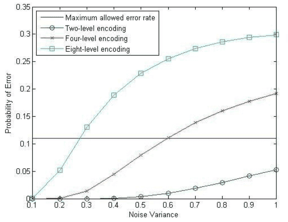
And this is the graph:

I hope that anyone in this forum may guide me to plot this graph.
Thank you.

 

[EngWiPy]

This thread fits better in the Electrical Engineering forum.

It is simpler to start with simplest case of binary input signals. In this case, you have two input signals $x_1$ and $x_2=-x_1$. The received signal over AWGN channel is given by $y=\pm x_1+n$, depending on which signal was actually transmitted. In this scheme, both signals are on the real line, and if they are equiprobable, then the decision boundary is at 0. This means that, the detector decides that the transmitted signal is $x_1$ if the received signal $y>0$, and it decides $x_2=-x_1$ if $y<0$. If $y=0$, then the receiver makes a fair coin guess. In this case, the probability or error is given by:

$$P(E)=P(E/x_1)p(x_1)+P(E/x_2)p(x_2)$$

where $P(E/x_k)$ is the probability of error given $x_k$ was transmitted, $p(x_k)$ is the probability of transmitting $x_k$. Let's compute $P(E/x_2)$:

$$P(E/x_2)=\text{Pr}\left[y>0/x_2\right]=\int_{0}^{\infty}p(y/x_2)\,dy=\frac{1}{\sqrt{2\pi\sigma_n^2}}\int_{0}^{\infty}\exp\left(-\frac{1}{2\sigma_n^2}(y+x_1)^2\right)\,dy=Q\left[x_1/\sigma_n\right]$$

where $Q[.]$ is the Q-function. If you assume that $x_1=1$, then the conditional probability of error can be written as

$$P(E/x_2)=Q\left[\frac{1}{\sqrt{\sigma_n^2}}\right]$$

You will get the same result for $P(E/x_1)$. So, assuming that $p(x_1)=p(x_2)=0.5$, the total probability of error will be

$$P(E)=0.5\times Q\left[\frac{1}{\sqrt{\sigma_n^2}}\right]+0.5\times Q\left[\frac{1}{\sqrt{\sigma_n^2}}\right]=Q\left[\frac{1}{\sqrt{\sigma_n^2}}\right]$$.

which can be plotted for different values of $\sigma_n^2$. In the case of more than 2 signals, you need to know the modulation technique (MPSK, MFSK, ... etc), and the decision boundaries between the signal points in the signal constellation. For that, refer to one of the textbooks like Digital Communications for John Proakis. But the steps are almost the same.

 

[Nur Ziadah]

This thread fits better in the Electrical Engineering forum.

It is simpler to start with simplest case of binary input signals. In this case, you have two input signals $x_1$ and $x_2=-x_1$. The received signal over AWGN channel is given by $y=\pm x_1+n$, depending on which signal was actually transmitted. In this scheme, both signals are on the real line, and if they are equiprobable, then the decision boundary is at 0. This means that, the detector decides that the transmitted signal is $x_1$ if the received signal $y>0$, and it decides $x_2=-x_1$ if $y<0$. If $y=0$, then the receiver makes a fair coin guess. In this case, the probability or error is given by:

$$P(E)=P(E/x_1)p(x_1)+P(E/x_2)p(x_2)$$

where $P(E/x_k)$ is the probability of error given $x_k$ was transmitted, $p(x_k)$ is the probability of transmitting $x_k$. Let's compute $P(E/x_2)$:

$$P(E/x_2)=\text{Pr}\left[y>0/x_2\right]=\int_{0}^{\infty}p(y/x_2)\,dy=\frac{1}{\sqrt{2\pi\sigma_n^2}}\int_{0}^{\infty}\exp\left(-\frac{1}{2\sigma_n^2}(y+x_1)^2\right)\,dy=Q\left[x_1/\sigma_n\right]$$

where $Q[.]$ is the Q-function. If you assume that $x_1=1$, then the conditional probability of error can be written as

$$P(E/x_2)=Q\left[\frac{1}{\sqrt{\sigma_n^2}}\right]$$

You will get the same result for $P(E/x_1)$. So, assuming that $p(x_1)=p(x_2)=0.5$, the total probability of error will be

$$P(E)=0.5\times Q\left[\frac{1}{\sqrt{\sigma_n^2}}\right]+0.5\times Q\left[\frac{1}{\sqrt{\sigma_n^2}}\right]=Q\left[\frac{1}{\sqrt{\sigma_n^2}}\right]$$.

which can be plotted for different values of $\sigma_n^2$. In the case of more than 2 signals, you need to know the modulation technique (MPSK, MFSK, ... etc), and the decision boundaries between the signal points in the signal constellation. For that, refer to one of the textbooks like Digital Communications for John Proakis. But the steps are almost the same.

Thank you EngWiPy for the explanation...I am sorry if my question is too simple. Is the $$Q\left[\frac{1}{\sqrt{\sigma_n^2}}\right]$$ same with the equation 4? Could you explain me what is the meaning of y and xi in the equation 4?
Thanks a lot sifu ;)

 

[EngWiPy]

Eq. 4 is the distribution of the received signal $y$, given that signal $x_i$ was transmitted, where $x_i$ can be any of the $M$ available input signals. So, what we want to find is, for a given received signal, what signal was transmitted, right? To find this, we need to find the signal that has the maximum conditional probability $p(x_i/y)=\frac{p(y/x_i)\,p(x_i)}{p(y)}$ using Bayes rule. But since all signals have the same probabilities $p(x_i)$, and $p(y)$ is common to all possible transmitted signals, the problem is reduced to finding the signal with the maximum $p(y/x_i)$.

The received signal is $y=x_i+n$, where $n$ is an additive white Gaussian noise with zero mean and variance $\sigma_n^2$. So, for a given $x_i$, $y$ becomes a Gaussian random variable with mean $x_i$ and a variance $\sigma_n^2$. Eq. 4 describes just this. How to find the transmitted signal that maximizes $p(y/x_i)$? Simple, find the signal point that is closest to $y$. Now, how to quantify the error probability, you need to follow the steps I showed.

So, to answer your question: Eq. 4 is the distribution of the received signal $y$, given $x_i$ was transmitted. Which means that, if you transmit $x_i$ over an AWGN channel a large number of times, the observed received signal at the receiver will follow a Gaussian distribution centered around $x_i$, with a variance equals to the noise variance. $Q\left[\frac{1}{\sqrt{\sigma_n^2}}\right]$ is that quantity that measures the probability of error. That is, if we transmit $x_i$ a large number of times, how many times from the total times $y$ won't be closest to $x_i$, which results in erroneous decision.

Hope this helps.

 

[Nur Ziadah]

Eq. 4 is the distribution of the received signal $y$, given that signal $x_i$ was transmitted, where $x_i$ can be any of the $M$ available input signals. So, what we want to find is, for a given received signal, what signal was transmitted, right? To find this, we need to find the signal that has the maximum conditional probability $p(x_i/y)=\frac{p(y/x_i)\,p(x_i)}{p(y)}$ using Bayes rule. But since all signals have the same probabilities $p(x_i)$, and $p(y)$ is common to all possible transmitted signals, the problem is reduced to finding the signal with the maximum $p(y/x_i)$.

The received signal is $y=x_i+n$, where $n$ is an additive white Gaussian noise with zero mean and variance $\sigma_n^2$. So, for a given $x_i$, $y$ becomes a Gaussian random variable with mean $x_i$ and a variance $\sigma_n^2$. Eq. 4 describes just this. How to find the transmitted signal that maximizes $p(y/x_i)$? Simple, find the signal point that is closest to $y$. Now, how to quantify the error probability, you need to follow the steps I showed.

So, to answer your question: Eq. 4 is the distribution of the received signal $y$, given $x_i$ was transmitted. Which means that, if you transmit $x_i$ over an AWGN channel a large number of times, the observed received signal at the receiver will follow a Gaussian distribution centered around $x_i$, with a variance equals to the noise variance. $Q\left[\frac{1}{\sqrt{\sigma_n^2}}\right]$ is that quantity that measures the probability of error. That is, if we transmit $x_i$ a large number of times, how many times from the total times $y$ won't be closest to $x_i$, which results in erroneous decision.

Hope this helps.

Thank you so EngWiPy..I get it now.