Implementing a weird-looking boundary condition (PDE/FDM)

In summary: The issue being faced is with the implementation of these boundary conditions, specifically at the corners of the domain. The solution method being used is Gauss-Seidel iteration, and the problem may lie in the corners of the domain, specifically at points (0,1) and (1,1). The correct boundary condition to use at these points is unclear.
  • #1
maistral
240
17
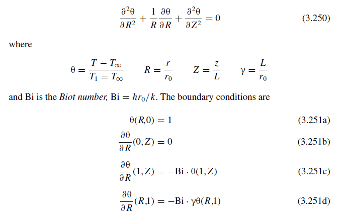
So I have this problem, taken from Kraus's heat transfer book.
63ye6d.png


So deriving the computational molecule, the conditions for (3.251a), (3.251b) is a bit of a no brainer. The issue I am having is about the boundaries for (3.251c) and (3.251d). This is actually the first time I have seen this kind of boundary condition.

How do I deal with this? My hypothesis is to integrate the equations (lol) but the constants of integration stay around... I have no idea what to do at all. Bi and γ are constants. Thanks!
 
Physics news on Phys.org
  • #2
Oh, to add.

There's an analytical expression for the solution; and I am able to graph the resulting multivariate graph. I intend to do the numerical analysis as another way of solving it. The problem is, even if I implement the 'integrating the boundary condition' part or if I use the ghost point strategy, both of it does not work - the graph from the numerical solution is way too far from the analytical expression's graph.
 
  • #3
You're solving this by finite difference, correct?
 
  • #4
Yes sir. Finite difference.
 
  • #5
$$\theta (1+\Delta R, Z)-\theta (1-\Delta R, Z)=-2(\Delta R) Bi\ \theta (1,Z)$$
so
$$\frac{\partial ^2 \theta}{\partial R^2}=2\frac{(\theta (1-\Delta R, Z)-\theta (1,Z))-(\Delta R) Bi\ \theta (1,Z)}{(\Delta R)^2}$$
or
$$\frac{\partial ^2 \theta}{\partial R^2}=2\frac{(\theta (1-\Delta R, Z)-\theta (1,Z))}{(\Delta R)^2}-2\frac{Bi\ \theta(1,Z)}{\Delta R}$$
or
$$\frac{\partial ^2 \theta}{\partial R^2}=2\frac{(\theta (1-\Delta R, Z)-[1+(\Delta R) Bi]\theta (1,Z))}{(\Delta R)^2}$$
 
  • #6
Thanks for replying sir. Actually I did it already, but I seem to be getting erroneous results. Could you have my computational molecules for each boundary checked first?

I intend to implement a solution similar to Gauss-Seidel iteration; thus I kept on factoring out the 'center' molecule.
 
Last edited:
  • #7
Sorry. I'll help with the finite differencing, but, as far as the debugging is concerned, you're on your own.
 
  • #8
Oh, it's alright sir.

Apparently my computational molecules for the boundaries are correct; but the numerical solution is still given different values. I'm starting to think that the problem comes from the corners - problem is what should I do with the corners (0,1) and (1,1). What boundary should I invoke? Say for the upper left corner (0,1); is it 3.251b or 3.251d?
 
  • #9
maistral said:
Oh, it's alright sir.

Apparently my computational molecules for the boundaries are correct; but the numerical solution is still given different values. I'm starting to think that the problem comes from the corners - problem is what should I do with the corners (0,1) and (1,1). What boundary should I invoke? Say for the upper left corner (0,1); is it 3.251b or 3.251d?
Both
 

1. What is a boundary condition in PDE/FDM?

A boundary condition is a set of conditions that are imposed at the boundaries of a domain in a partial differential equation (PDE) or finite difference method (FDM) problem. These conditions specify how the solution should behave at the boundaries of the domain.

2. How do you implement a weird-looking boundary condition in PDE/FDM?

Implementing a weird-looking boundary condition in PDE/FDM involves modifying the equations and algorithms used to solve the problem. This can include adding additional terms or constraints to the equations, or using specialized numerical methods to handle the unusual boundary condition.

3. What are some examples of weird-looking boundary conditions in PDE/FDM?

Some examples of weird-looking boundary conditions in PDE/FDM include non-linear or non-local boundary conditions, conditions that vary with time or space, and conditions that involve derivatives of the solution at the boundary.

4. What are the challenges of implementing a weird-looking boundary condition in PDE/FDM?

The main challenge of implementing a weird-looking boundary condition in PDE/FDM is that it may require more complex mathematical and numerical techniques, which can be difficult to implement and may result in slower computation times. Additionally, the boundary condition may introduce instability or convergence issues in the solution.

5. How can I verify the accuracy of my implementation of a weird-looking boundary condition in PDE/FDM?

To verify the accuracy of your implementation, you can compare your results to analytical solutions, if available. You can also perform convergence tests by refining the grid or changing the timestep and observing how the solution changes. Additionally, you can compare your results to other published solutions or use benchmark problems to validate your implementation.

Similar threads

  • Differential Equations
Replies
9
Views
2K
Replies
4
Views
1K
  • Differential Equations
Replies
2
Views
2K
Replies
1
Views
1K
Replies
8
Views
2K
  • Differential Equations
Replies
8
Views
4K
  • Differential Equations
Replies
5
Views
2K
  • Differential Equations
Replies
1
Views
2K
Replies
5
Views
2K
  • Differential Equations
Replies
1
Views
2K
Back
Top