Infinite Square Well with an Oscillating Wall (Klein-Gordon Equation)

[Foracle]

TL;DR

Numerical solution of the wavefunction blows up when the frequency of oscillation of the wall is high. What does this mean?

I am trying to numerically solve (with Mathematica) a relativistic version of infinite square well with an oscillating wall using Klein-Gordon equation. Firstly, I transform my spatial coordinate $x \to y = \frac{x}{L[t]}$ to make the wall look static (this transformation is used a lot in solving non-static boundary condition in the non-relativistic case), which brings Klein-Gordon equation to :
Input :

Output :

All constants have been set to 1

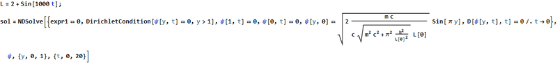
I tried to solve this system where $L(t)=2+sin(1000 t)$ using NDSolve :

Then I plot my result as a function of $(y,t)$ :

The wavefunction $\psi$ blows up. This doesn't happen when I tune the frequency down to 1, $L(t)=2+sin(t)$

My question is why does $\psi$ blow up when the frequency of the oscillation is high and what does it mean? Does it have anything to do with particle production? Or did I just mess up my code?

 

[Foracle]

I have located my error. It was the fact that when I set $\omega$ to 1000, the velocity of the wall, $\dot{L} = \omega cos(\omega t) \ge 1$, which is not allowed in the units that I am working with $(c=1)$.
The solution to this is just to set $L(t) = \frac{1}{\omega} (2+sin(\omega t))$, and this disastrous result doesn't happen anymore.