Interpreting VIA PCB characteristics through TDR and TDT

  • Thread starter yefj
  • Start date
23 replies · 5K views · last reply
yefj
Messages
166
Reaction score
2
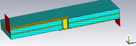
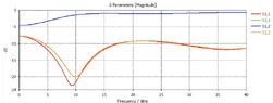
Hello ,I have simulated a basic VIA (shown in the photo) in CST EM simulator from 0 to 40GHz and extracted its attached S2P.
using the code below I resampled it and made IFFT with multiplied the normalised hamming window.
I got the following plots in MATLAB.
Is there a way to interpret the VIA properties threw these TRT and TDR plots?
Thanks.
Code:
clear all
Sp = sparameters('via.s2p');
Sp.Parameters(1,1,1)=0;
freqs=Sp.Frequencies; %40000X1
s11_half=Sp.Parameters(1,1,:);
s21_half=Sp.Parameters(2,1,:);
if freqs(1) ~= 0
           s11_dc = interp1(freqs, s11, 0, 'linear', 'extrap');
end

left_side=squeeze(s11_half);
left_side_s21=squeeze(s21_half);

% ===== Resample to uniform frequency grid =====
fi = linspace(freqs(1), freqs(end), length(freqs)).'; %40000X1
s11_resamples = interp1(freqs, left_side, fi, 'linear');
s21_resamples = interp1(freqs, left_side_s21, fi, 'linear');
right_side_miror=conj(s11_resamples(end-1:-1:2));
right_side_miror_s21=conj(s21_resamples(end-1:-1:2));
s11_full=[ s11_resamples;right_side_miror];
s21_full=[ s21_resamples;right_side_miror_s21]; %%


w = ifftshift(hamming(length(s11_full),'periodic'));
w=w./max(w);

%%%%%%%%%%%%%
df = fi(2) - fi(1);
N = length(s11_full);
t = (0:N-1).' / (N * df);   % time axis

rho = cumsum(real(ifft(s11_full.*w)));
z = (1+rho)./(1-rho)*50;

figure;
plot(t*1e12, z);
xlim([-100 450]);
xlabel('time [ps]');
title('TDR(reflection)');


figure;
plot(t*1e12, cumsum(real(ifft(s21_full.*w))));
grid on; grid minor; set (gca, 'gridalpha', 0.2); set(gca, 'minorgridalpha', 0.05);
xlim([0 1000]);
xlabel('time [ps]');
title('TDT(transmission)');
 
Attachments
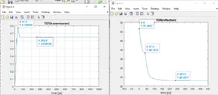
  • Two MATLAB figures side by side: left, 'TDT(transmission)' plotting a rising curve against time in ps, peaking near 0.77 at 37.5 ps and settling near 0.65; right, 'TDR(reflection)' plotting impedance falling from about 51.5 at 0 ps to about 23 by 237.5 ps.
    Capture.webp
    19.9 KB · Views: 20
  • 3D render of a simulated stripline-style PCB via: a cyan dielectric block with horizontal layer lines, a teal top ground plane, yellow signal traces and a yellow vertical via with red ground-wall fins at each end.
    3D_shape.webp
    20.2 KB · Views: 27
  • Line plot titled S-Parameters [Magnitude], dB against Frequency in GHz from 0 to 40. S1,2 starts near -4.5 dB and rises to about -1 dB. S1,1 and S2,2 dip to about -23 dB and -20 dB near 9.5 GHz, then recover to about -11.5 dB at 40 GHz.
    S_param.webp
    21.5 KB · Views: 33
Hello , I have resimulated the structure in another way and got a result much better to realistic DC value
s-parameters .
I made again IFFT to the S2p file and got the attached plots.

given my situation few questions:
1.given my 40GHz BW what kind of sizes I can use TDR TRT effectively
2.given my new IFFT plots is how can I see the geometrical properties of the VIA in them?
Is there some intuitions?

Line plot titled TDT(transmission) showing the time-domain transmission rising from 0 at 0 ps to about 1.0 by roughly 100 ps, then flat to 1000 ps. Axes: time [ps] 0 to 1000, amplitude 0 to 1.2.

Line plot titled TDR(reflection) of impedance in ohms against time in ps from 0 to 450, showing a sharp dip near 25 ps and a peak near 38 ps, then settling to about 47.5 ohms after roughly 100 ps.

Line graph of S-parameters magnitude in dB versus frequency from 0 to 40 GHz; S1,1 and S2,2 dip near 11 GHz to about -43 dB, S1,2 and S2,1 stay near 0 dB.
 
yefj said:
Is there a way to interpret the VIA properties threw these TRT and TDR plots?
You have two tracks with known impedance, joined through the PCB by a short cylindrical via. The via will probably not match the impedance of the tracks, so it will appear to be a quarter wave transformer with the via length, adjusted for velocity factor √Er.

Usually, only ground and power are routed through vias, and then through multiple parallel vias. It is not good practice to run signals through vias, at microwave frequencies. Keep signals in the signal plane, between or above ground plane(s).

My guess is that the via will appear to be a short cylindrical transmission line, probably inductive. You should be able to see the length of the via in the wavelength of the highest transmission frequency, and the impedance of the via in the TDR. Thinner vias are more inductive, so you may be able to adjust the via diameter until it matches the track impedance on both sides of the PCB. Feathering the track as it approaches the via, may ease reflection from the transition. To get a first approximation, compute the impedance of the via as a longer cylindrical transmission line.
 
yefj said:
I have simulated a basic VIA (shown in the photo)
3D render of a stacked multilayer PCB cross-section with teal copper planes, cyan dielectric layers, yellow traces and a yellow vertical via with red side walls at each end.


What you show is a 3-layer PCB, which is not used in practice.

Baluncore said:
It is not good practice to run signals through vias, at microwave frequencies. Keep signals in the signal plane, between or above ground plane(s).
This point made by @Baluncore should be emphasized. It is generally a design error to run high-frequency signals through vias, since the resulting ##Z_0## is not constant and does not match the transmission line. The transmission line physical structure and resulting ##Z_0## need to be maintained throughout the length of the TL from the transmit gate to the receive gate(s). Also, the TL must be properly terminated to avoid ringing (either forward-terminated for point-to-point TLs with a single receive gate, or back-terminated for TLs that have several receive gates).

Back in the early days of the FCC imposing EMI limits on electronic devices (like in the mid-1980s), one of the biggest problems in quieting down digital PCBAs was that little attention was paid to the routing of fast digital traces, and the resulting ringing from all the ##Z_0## mismatches caused lots of unintentional radiation from the PCBAs and the product enclosures and cables. [1]

Note also that this constant ##Z_0## requirement means that the TL signal trace should not pass close to other traces or grounded features, since this can also alter the ##Z_0## value.

[1] High Speed Digital Design, A Handbook of Black Magic, by Howard W. Johnson and Martin Graham, Chapter 7 on Vias, PTR Prentice Hall, 1993.
 
Last edited:
Hello, My goal is to learn to read TDT TRT and to see as much as possible about a VIA.
this imaginary PCB simulation is only an example for me to learn via responce in TDR.
later I will build multilayer VIA PCB.

few questions:
can I see threw tdr tdt responces peaks if its inductive or capacitative peak?
Is there mathematics explaining this?

can I see VIA structure properties threw the peaks of the TDT and TDR?
Thanks.
 
yefj said:
can I see threw tdr tdt responces peaks if its inductive or capacitative peak?
The "TD" in TDR refers to the time domain (Time Domain Reflectometer). It measures reflections in the time domain as seen at the transmitting port.
 
Hello , Yes I know what TDR is I need to know how to interpret its capacitance inductance. parts.
how do i do that?
can I see VIA structure properties threw the peaks of the TDT and TDR?
 
The direction of the reflection (adding or subtracting from the transmitted pulse) will tell you if the ##Z_0## mismatch at the via is positive or negative. From that you can probably infer whether it is inductive or capacitive. Most likely the ##Z_0## mismatch of the via will look positive/inductive in nature.
 
Hello,can you give me some manual regarding how to mathemtickally we prove that the reflection is capacitative or iductive?
 
yefj said:
can I see VIA structure properties threw the peaks of the TDT and TDR?
BTW, do you want me to fix the "TRT" in your thread title to "TDT"?
 
Yes sorry for the mistake.
Sorry for the stupid question but I know that I can get reflection coeffient threw the TDR by the formula below .
but how can I know that out ZL is inductive or capacitative?
Zc=1/jwc ZL=jwl
these formulas dont help me understand this in the wiki link you posted.
Equation: Gamma = (Z_L - Z_0) / (Z_L + Z_0), with a trailing period, written on a dark background.
 
I am trying to simulate time domain reflectometry and recognise threw the pulse responce if the load is capacitative or inductive.
As you can see its not working .
Where did I go wrong with the concept.
what is the proper way to see threw the time responce if the load is capacitative or inductive?
LTspice simulation: schematic of a 1 V pulse source V1 driving series resistor R1 (100) to an inductor L1 (100p) with .tran 100p, above plots of V(in) as a 1.0 V pulse and V(out) showing a positive spike near 10 ps decaying to about -80 mV, then a negative spike near 60 ps.
LTspice simulation: top plot shows V(in) pulse rising 0 to 1.0V and falling back, and V(out) rising in a ramp from 0 to about 5.5mV over 0 to 100ps; bottom shows schematic of V1 PULSE source, R1 100 ohm, and C1 100p from Out to ground.
 
TDR is a plot of impedance (driver voltage) against reflection time.
Z = √( L / C )
You cannot say if it is the inductance or the capacitance of the transmission line that has changed, only that the ratio and resulting impedance has changed.

There is an HP beginners guide to TDR here.
HP Application Note 62. Time Domain Reflectometry.
https://hparchive.com/Application_Notes/HP-AN-62.pdf

yefj said:
As you can see its not working.
During the pandemic, I wrote a TDR simulation in LTspice, when students could not get to the lab, so needed to simulate the practical. I will see what I can find from back then in the archives.
 
  • Like
Likes   Reactions: DaveE and berkeman
Here is a simple TDR simulated in LTspice.
Remove the .txt extensions from both files, then run the LTspice file.asc
Start by changing the termination impedance and notice how the Vin changes later due to the reflection.
 
Attachments
This LTspice model is sufficient to model the signal passing through a via.
T1 is the line on one side of the PCB. T2 will become the via, if it is shortened. T3 is the line on the opposite side of the PCB. Values that are unusual are marked with an asterisk, so they will not be missed or forgotten.
LTspice schematic of a transmission-line chain: a 50R driver resistor R1 and pulse source V1 feed T1 (Td=1u, Z0=50), T2 (Td=0u5, Z0=70), and T3 (Td=1u, Z0=50), ending at a 5n capacitor C1 and a 60R load R2 labelled termination impedance.

This is the TDR response due to the T2 (via) impedance and the capacitive termination.
LTspice simulation plot of TDR waveforms: green V(source) steps to 1.0V near 0 µs, yellow V(in) rests at 0.5V with a downward pulse near 5 µs, red V(out) rises from 0V near 2.5 µs and settles near 0.55V.

The green shows the driver pulse, the yellow the TD reflected signal, and the red the destination signal. TDR times are twice the transit times.

Notice how T2, the higher impedance line, shows as a higher voltage.
Notice how the capacitive load shows as a downward pulse, series inductance would make a positive pulse.
Notice the final output voltage settles to slightly greater than 0.5V, because the termination resistance is greater than 50R.

Following the capacitive pulse in the TDR, are secondary echos of the capacitive pulse in both end mismatches of T2, first positive, then negative. Change Zo of T2 to say 40R, so the T2 voltage will step down, and see those two echos invert.

This model shows how TDR can look down a line at impedance discontinuities, and how the reflection can be interpreted. That will give you an understanding of TDR. To model a real via using this schematic, you will need to significantly shorten the length of T2, and greatly reduce the rise time of the test pulse. Short TLs, and fast rise-times, will slow down the simulation.

The two text files are the source LTspice files, wrapped so they can be attached to this thread, then downloaded and run.
 
Attachments
Hello Baluncore,regarding this good simulation, few questions:
1.The most important is,How do you see that the echo from the right side and the left side of the T2?
How do you distinguish between them and spot the source of the discontinuety purely from a ripple in the time domain? could you please give some graphical or mathematical intuition?
"Following the capacitive pulse in the TDR, are secondary echos of the capacitive pulse in both end mismatches of T2, first positive, then negative. Change Zo of T2 to say 40R, so the T2 voltage will step down, and see those two echos invert."

2. why did you terminate with 60Ohm in parralel with 5nF.
3.I know that phase velicity*round_trip_time*0.5 is the distance.we dont have phase velocity.
so If I want to locate my via in the PCB ,how do I convert this ltspice time delay into distance?
 
I think I should answer your questions backwards.
yefj said:
3. I know that phase velicity*round_trip_time*0.5 is the distance. we dont have phase velocity. so If I want to locate my via in the PCB ,how do I convert this ltspice time delay into distance?
LTspice models the specified circuit parameters against time. It does not model physical dimensions, so for LTspice transmission line models, you must specify the time delay. The physical length and the velocity factor are irrelevant to LTspice.
Knowing the velocity factor vf, and the speed of light c = 299 792 458 ;
Time = Length / ( vf * c ) ;
Length = Time / ( vf * c ) ;
Where time is in seconds, and length is in metres.

yefj said:
2. why did you terminate with 60Ohm in parralel with 5nF.
Because it demonstrates the negative kick of a capacitor, and how the final termination impedance of the line controls the final voltage in the TDR. You need to play with the parameters to see what changes.

yefj said:
How do you distinguish between them and spot the source of the discontinuety purely from a ripple in the time domain? could you please give some graphical or mathematical intuition?
That is not "ripple in the time domain", it is the "sum of all echos", from all mismatches, many times. As the pulse reaches each discontinuity, it is split into two, being reflected backwards by the reflection coefficient, and passed forward by the transmission coefficient. Both those signals are then reflected and transmitted, making two more pulses each time they encounter a mismatch. It is that binary tree of split signals, going all possible ways, that makes the network look like a hall of mirrors. If the line is not specified as lossy, the energy in the line will be gradually be lost in the far line termination, or the source impedance of the generator.

yefj said:
1.The most important is,How do you see that the echo from the right side and the left side of the T2?
The negative kick from the capacitor is a pulse that travels back to the viewer via the echo chamber of all the mismatches between all the lines. You need to experiment with the parameters to understand the implications, and see the patterns.

In our universe we only see reflections from mismatches of impedance. We cannot see the inside of a glass prism, or of a lossless transmission line.
 
Hello Baluncore ,regarding your good explanantions Two questions:
1. I have made the three transmission line 50Ohms and kept the capacitative mismatch as shown in the photo below.Two questions:
Why on the "out" node there is no negative kick unlike "left" and "right" nodes?


2.regarding the "hall of mirrors", I made a situation where I matched the load and done mismatch in T2 as shown in the second photo.
I know that At first "left" node sees a pulse then the second rise is because a while its a round trip of 30-50 impedance mismatch. the round trip is 1u so the distance is 0.5u as defined in the T2.So I can handle understanding one reflection

When I intreduce the load mistach and I will have double mismatch and there will be a binary tree of reflections.
How can I analyse the time domain plot and see the binary tree reflecrtion structure.
Is there a basic graphical example so I can see the logic of lookind at the pulse and see its "origins"?
Updated Ltspice file as TXT is attached.
Thanks.

LTspice schematic of a 50 ohm transmission line chain: source V1 with R1 50R driver, lines T1 and T2 (Td=0u5 Z0=50) and T3, capacitor C1 5n and R2 60 at the out node, plus simulation waveforms of V(in), V(out), V(source) and V(right) over time.

LTspice simulation schematic: source V1 with pulse through R1 50R driver, then lines T1, T2 (Z0=30) and T3 (Z0=50) to termination R2 50, with probe traces above showing V(source), V(left) and V(right) over 10 us.
LTspice schematic and simulation of a 50 ohm transmission line chain: source V1 with R1 50R driver, lines T1 and T3 at Z0=50, middle line T2 at Z0=30, load R2 50, with waveforms of source, left, and right nodes plotted above.
 
Attachments
The network is drawn across the top. The TDR plot is down the LHS, showing how multiple transmissions and reflections sum.
Bounce (lattice) diagram of a transmission line with source, line 1, line 2, line 3 and termination columns, with time labels in microseconds from 0.0 to 6.0 us tracing repeated reflections.
 
Hello Baluncore,I have made the three transmission line 50Ohms and kept the capacitative mismatch as shown in the photo below.
Why on the "out" node there is no negative kick unlike "left" and "right" nodes?"
Thanks.
LTspice schematic of three 50 ohm transmission lines T1, T2 and T3 with a 5n capacitor C1 and 60 ohm R2 at the out node, above waveform plots of source, left, right and out voltages.
 
yefj said:
Why on the "out" node there is no negative kick unlike "left" and "right" nodes?"
When the three TLs have the same impedance they look like a single line. Although you can plot V(left) and V(right), there can be no reflection at those nodes because they are matched.

At V(left) and V(right) you are watching the step move towards the termination, then later, the reflection heading back towards the source. V(out) is the sum of both the incident signal, and its reflection, at the capacitor, with no separation in time or direction.