yefj
- 64
- 2
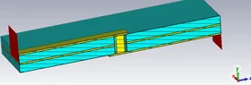
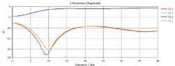
Hello ,I have simulated a basic VIA (shown in the photo) in CST EM simulator from 0 to 40GHz and extracted its attached S2P.
using the code below I resampled it and made IFFT with multiplied the normalised hamming window.
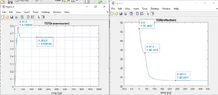
I got the following plots in MATLAB.
Is there a way to interpret the VIA properties threw these TRT and TDR plots?
Thanks.
using the code below I resampled it and made IFFT with multiplied the normalised hamming window.
I got the following plots in MATLAB.
Is there a way to interpret the VIA properties threw these TRT and TDR plots?
Thanks.
Code:
clear all
Sp = sparameters('via.s2p');
Sp.Parameters(1,1,1)=0;
freqs=Sp.Frequencies; %40000X1
s11_half=Sp.Parameters(1,1,:);
s21_half=Sp.Parameters(2,1,:);
if freqs(1) ~= 0
           s11_dc = interp1(freqs, s11, 0, 'linear', 'extrap');
end

left_side=squeeze(s11_half);
left_side_s21=squeeze(s21_half);

% ===== Resample to uniform frequency grid =====
fi = linspace(freqs(1), freqs(end), length(freqs)).'; %40000X1
s11_resamples = interp1(freqs, left_side, fi, 'linear');
s21_resamples = interp1(freqs, left_side_s21, fi, 'linear');
right_side_miror=conj(s11_resamples(end-1:-1:2));
right_side_miror_s21=conj(s21_resamples(end-1:-1:2));
s11_full=[ s11_resamples;right_side_miror];
s21_full=[ s21_resamples;right_side_miror_s21]; %%


w = ifftshift(hamming(length(s11_full),'periodic'));
w=w./max(w);

%%%%%%%%%%%%%
df = fi(2) - fi(1);
N = length(s11_full);
t = (0:N-1).' / (N * df);   % time axis

rho = cumsum(real(ifft(s11_full.*w)));
z = (1+rho)./(1-rho)*50;

figure;
plot(t*1e12, z);
xlim([-100 450]);
xlabel('time [ps]');
title('TDR(reflection)');


figure;
plot(t*1e12, cumsum(real(ifft(s21_full.*w))));
grid on; grid minor; set (gca, 'gridalpha', 0.2); set(gca, 'minorgridalpha', 0.05);
xlim([0 1000]);
xlabel('time [ps]');
title('TDT(transmission)');