Linearization of a function error viewed with differentials

[mcastillo356]

TL;DR Summary

Can't assume a premise of the reasoning

Hi, PF, want to know how can I go from a certain error formula for linearization I understand, to another I do not

Error formula for linearization I understand:

If $f''(t)$ exists for all $t$ in an interval containing $a$ and $x$, then there exists some point $s$ between $a$ and $x$ such that the error $E(x)=f(x)-L(x)$ in the linear approximation $f(x)\approx{L(x)=f(a)+f'(a)(x-a)}$ satisfies

$E(x)=\dfrac{f''(s)}{2}(x-a)^2$

(...)

Quote I don't understand:

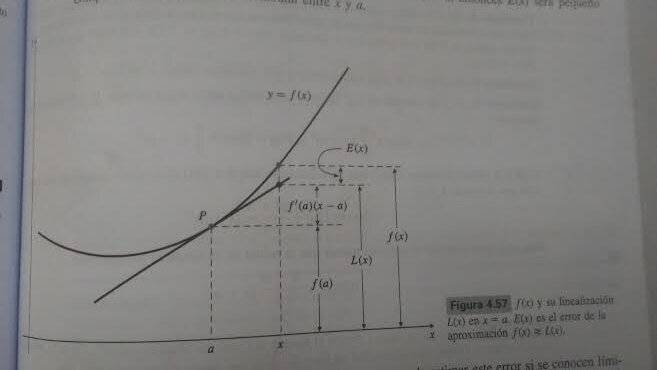
The error in the linearization of $f(x)$ about $x=a$ can be interpreted in terms of differentials (...) as follows: if $\Delta x=dx=x-a$, then the change in $f(x)$ as we pass from $x=a$ to $x=a+\Delta x$ is $f(a+\Delta x)-f(a)=\Delta y$, and the corresponding change in the linearization $L(x)$ is $f'(a)(x-a)=f'(a)dx$, which is just the value at $x=a$ of the differential $dy=f'(x)dx$. Thus,

$E(x)=\Delta y-dy$

The error $E(x)$ is small compared with $\Delta x$ as $\Delta x$ approaches 0, as seen in Figure.

Attempt to understand $E(x)=\Delta y-dy$:

In any approximation, the error is defined by

error=true value-approximate value

If the linearization of $f$ about $a$ is used to approximate $f(x)$ near $x=a$, that is,

$f(x)\approx{L(x)=f(a)+f'(a)(x-a)}$

then the error $E(x)$ in this approximation is

$E(x)=f(x)-L(x)=f(x)-f(a)-f'(a)(x-a)$

It is the vertical distance at $x$ between the graph of $f$ and the tangent line to that graph at $x=a$, as shown in Figure. Observe that if $x$ is "near" $a$, then $E(x)$ is small compared to the horizontal distance between $x$ and $a$

$\displaystyle\lim_{\Delta x \to{0}}{\dfrac{\Delta y -dy}{\Delta x}}=\displaystyle\lim_{\Delta x \to{0}}{\left({\dfrac{\Delta y}{\Delta x}-\dfrac{dy}{dx}}\right)}=\dfrac{dy}{dx}-\dfrac{dy}{dx}=0$

Well, actually is a fake attempt: either of the limits tend to zero when $\Delta x\rightarrow{0}$, but I'm confused by the premise of reasoning:
$\Delta x=dx=x-a$. Is there any explanation for a dummy like me? I fear the answer might need non standard analysis. But the premise sounds like "if apple=pear=apple".

 

[hutchphd]

I am not sure I understand the question. That being said I believe your equivalence follows rom the Mean Value Therorem. ( There will always be a point s within the interval where the definitions coincide...is that the question?)

 

[mcastillo356]

I am not sure I understand the question. That being said I believe your equivalence follows rom the Mean Value Therorem. ( There will always be a point s within the interval where the definitions coincide...is that the question?)

@hutchphd, I've intentionally put a lightbulb to your response; now, the fact is that past year I was an undergraduate in Physics. I chose UNED
https://en.wikipedia.org/wiki/National_University_of_Distance_Education
because it offered me the possibility of making my desire to learn compatible with the lack of time; to the point, and out of the pot: I want a good introductory book to non-standard analysis.
Sorry, that is the question I should have asked.
I prefer English, I manage better.
Love

 

[Svein]

Summary:: Can't assume a premise of the reasoning

If exists for all in an interval containing and , then there exists some point between and such that the error in the linear approximation satisfies

Not quite true, you must also assume that f'' is continuous.

 

[mcastillo356]

Not quite true, you must also assume that f'' is continuous.

@Svein, my personal opinion is that if $f''(t)$ exists for all $t$ in an interval containing $a$ and ##x#, shoudn't be continuous in that interval, understanding it's a linearization?

 

[Svein]

Try this example: Let f be given as $f(x)=-x^{2}(x<0);x^{2}(x\geq 0)$. Then $f''(x)$ is discontinuous at x=0.

 

[PeroK]

@Svein, my personal opinion is that if $f''(t)$ exists for all $t$ in an interval containing $a$ and ##x#, shoudn't be continuous in that interval, understanding it's a linearization?

That is equivalent to saying that all derivatives are continuous.

 

[mcastillo356]

I am not sure I understand the question. That being said I believe your equivalence follows rom the Mean Value Therorem. ( There will always be a point s within the interval where the definitions coincide...is that the question?)

@hutchphd, sorry, rom means right or maybe?

Not quite true, you must also assume that f'' is continuous.

@Svein, I've been wondering...Well, I'm talking nonsense for sure, but this is what I've done: take $y=\dfrac{1}{x}$, which is discontinous at $x=0$; compute the first and the second integral with an online calculator, and now I think: $g=x(\ln{(|x|-1)}$ is not linearizable?. It is. But the second derivative is not continuous in $\Bbb{R}$. I can't tell I must assume it. I apologize in advance.

That is equivalent to saying that all derivatives are continuous.

Wise remark. And true. I mean I'm stucked.

Love

 

[hutchphd]

@hutchphd, sorry, rom means right or maybe?

My apologies its just a typo: from

 

[Svein]

compute the first and the second integral with an online calculator, and now I think: is not linearizable?. It is.

No. $\ln(\vert x\vert )$ does not exist at x=0 (in popular terms: it goes to -∞).

 

[mcastillo356]

Could it be something like this?

Not quite true, you must also assume that f'' is continuous.

Yes.
To get to $E(x)=\dfrac{f''(s)}{2}(x-a)^2$, which is an error formula for linearization if we know bounds for the second derivative of $f$, it is needed to apply twice the Mean Value Theorem: "Suppose that the function $f$ is continuous on the closed, finite interval $[a,b]$ and it is differentiable on the open interval $(a,b)$...Is this the right way?

 

[mathwonk]

It seems the error term in post #1 is valid if only the second derivative exists, even if not continuous. See Courant, vol 1, p. 324, footnote, for example. This extends (and uses) the mean value theorem, where only the existence of the derivative is required. The continuity of the second derivative is apparently used to deduce the more precise integral form of the error term.

One consequence of this interesting property of the derivative is that it satisfies the intermediate value property even if not continuous. I.e. if the derivative of a function is negative at one point of an interval, and positive later, it implies that the function is not monotone, but changes direction, and a function that changes direction between two points must have a local extremum between them, hence the derivative, if it exists, must be zero there.

We often think intuitively of the intermediate value property as equivalent to continuity, but technically it is slightly weaker. This distinction is sometimes blurred in some less precise discussions, and in fact, continuity is (incorrectly to a mathematician) "defined" by this property on page 6 of the prelilminary section of volume one of Maxwell's Treatise on electricity and magnetism.

 

[mcastillo356]

It seems the error term in post #1 is valid if only the second derivative exists, even if not continuous. See Courant, vol 1, p. 324, footnote, for example.

Sorry, I don't find the quote. Could you give me more details?
Your posts have been very educational, thanks!

 

[Frabjous]

Sorry, I don't find the quote. Could you give me more details?
Your posts have been very educational, thanks!

Here you go

 

[mathwonk]

Here is another discussion of the proof in more detail:
https://gowers.wordpress.com/2014/02/11/taylors-theorem-with-the-lagrange-form-of-the-remainder/

See also the comment near the end of the comments section, where a simpler version of the proof is given, from a book used in Flanders, Belgium.

A similar proof appears on pages 494-495 of Calculus of one variable, by Joseph Kitchen, Addison Wesley 1968.

The "usual" proof, using Cauchy's mean value theorem which Tim Gower complains about in the link above to his blog, is on pages 345-7 of Spivak's famous Calculus book.