Prove It
Gold Member
MHB
- 1,434
- 20
Reading the Integral Calculus tutorial, I felt like contributing. Do with it what you wish...
Proposition: You can evaluate areas exactly using Integrals.
Knowing that an integral is an antiderivative, and that derivatives are RATES, it seems odd that going in reverse would give geometric measurements.
To prove this proposition, we need to do some analysis of functions in general.First, we should note that a function can reach its global maxima and minima only at turning points and endpoints.
Theorem 1: The Extreme Value Theorem (given without proof due to how obvious it seems).
The Extreme Value Theorem states that for any function $\displaystyle f(x) $ defined over an interval $ \displaystyle x \in [\alpha, \beta]$ and continuous over $\displaystyle x \in (\alpha, \beta ) $, it must reach its maximum and minimum at some points in $\displaystyle x \in [\alpha, \beta]$Theorem 2: Rolle's Theorem (also obvious, but the proof follows nicely from the Extreme Value Theorem).
Rolle's Theorem states that if a function is defined over $\displaystyle x \in [a,b] $ and is continuous over $\displaystyle x \in (a, b)$, if the function has the same value at two points, i.e. if $\displaystyle f(a) = f(b) $, then there must be a turning point in between them, since at some point between them the function has to turn to go back to that function value.
Therefore, if $\displaystyle f(a) = f(b) $, then there exists some $\displaystyle c \in [a, b] $ such that $\displaystyle f'(c) = 0 $.
Proof: If the function's endpoints are $\displaystyle a, b $ and we have $\displaystyle f(a) = f(b) $, then if $\displaystyle f(a) $ is a global minimum, so is $\displaystyle f(b) $, and if $\displaystyle f(a) $ is a global maximum, so is $\displaystyle f(b) $. But by the Extreme Value Theorem, the function must reach its global maximum and minimum at some points in the interval. If $\displaystyle f(a) = f(b) $ is the global maximum, then there must be a turning point as the global minimum. If $\displaystyle f(a) = f(b) $ is the global minimum, then there must be a turning point as the global maximum. If $\displaystyle f(a) = f(b) $ is neither the global maximum or minimum, then there must be two turning points as the global maximum and minimum. Q.E.D.Theorem 3: The Mean Value Theorem
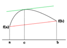
The Mean Value Theorem states that for any continuous and differentiable function over $\displaystyle x \in [a, b] $, the gradient of the chord between $\displaystyle a $ and $\displaystyle b $ is equal to the gradient of the tangent to the function at some point in between $\displaystyle a $ and $\displaystyle b $.
In symbols: $ \displaystyle \frac{f(b) - f(a)}{b - a} = f'(c) $ for some $\displaystyle c \in [a, b] $
Proof (from Wikipedia):
Define $\displaystyle g(x) = f(x) − rx $, where $r$ is a constant. Since $f$ is continuous on $[a, b]$ and differentiable on $(a, b)$, the same is true for $g$. We now want to choose $r$ so that $g$ satisfies the conditions of Rolle's theorem. Namely
\[ \displaystyle \begin{align*} g(a) &= g(b) \\ f(a) - r\,a &= f(b) - r\,b \\ r(b - a) &= f(b) - f(a) \\ r &= \frac{f(b) - f(a)}{b - a} \end{align*} \]
By Rolle's theorem, since $g$ is continuous and $g(a) = g(b)$, there is some $c$ in $(a, b)$ for which $\displaystyle g'(c) = 0 $, and it follows from the equality $g(x) = f(x) − r\,x$ that
\[\begin{align*}\displaystyle g'(x) &= f'(x) - r \\ g'(c) &= f'(c) - r \\ 0 &= f'(c) - r \\ r &= f'(c) \\ \frac{f(b) - f(a)}{b - a} &= f'(c) \end{align*}\]
as required. Q.E.D.Note, we can rearrange the equation from the Mean Value Theorem as $\displaystyle f(b) - f(a) = (b - a)f'(c) $. We will refer back to this later. Now to prove our original proposition...
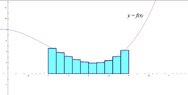
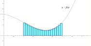
If we want to evaluate the area underneath a function $\displaystyle f(x) $ between $\displaystyle x = a $ and $\displaystyle x = b $. Start by making $\displaystyle n $ subdivisions on your interval and marking the midpoint of each, so that $\displaystyle a = x_0 < m_1 < x_1 < m_2 < x_2 < \dots < m_n < x_n = b $.
Then rectangles can be drawn of length $= x_i - x_{i-1}$ and width $= f(m_i)$, so that their area $= (x_i - x_{i-1})\,f(m_i)$.
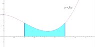
Then the area bounded by the curve and the $x$ axis between $x = a$ and $x = b$ can be approximated as $ \displaystyle A \approx \sum_{i = 1}^n \,(x_i - x_{i-1})\,f(m_i) $.
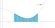
By making more subdivisions (making $n \to \infty$), this sum converges upon the true area.
So $ \displaystyle A = \lim_{n \to \infty} \sum_{i = 1}^n \,(x_i - x_{i-1})\,f(m_i).$
If we define $f(x)$ as the derivative of another function $F(x)$, the summand can be simplified using the Mean Value Theorem. In other words $\displaystyle F'(x) = f(x) \,\,\,\,\,\textrm{or}\,\,\,\,\, F(x) = \int{f(x)\,dx}$.
Remembering from the Mean Value Theorem that $(b-a)\,f'(c) = f(b) - f(a)$ for some $c \in (a,b)$, that means by making $n \to \infty$, the midpoint of each interval will become the only point in between each subinterval, and thus $\displaystyle (x_i - x_{i-1})\,f(m_i) = F(x_i) - F(x_{i-1}) $.
Substituting into the formula for the area gives
\[ \displaystyle \begin{align*}
A &=\lim_{n \to \infty}\sum_{i = 1}^n \,(x_i - x_{i-1})\,f(m_i)\\
&= \lim_{n \to \infty}\sum_{i = 1}^n\, \left[F(x_i) - F(x_{i-1})\right]\\
&= \lim_{n \to \infty} \left\{\, \left[F(x_1) - F(x_0)\right]+\left[F(x_2) - F(x_1)\right]+ \left[ F(x_3) - F(x_2) \right] + \dots + \left[ F(x_n) - F(x_{n-1}) \right] \right\} \\
&= \lim_{n \to \infty} \left[ F(x_n) - F(x_0) \right] \\
&= F(x_n) - F(x_0) \\
&= F(b) - F(a) \end{align*}\]So, in order to exactly evaluate the area underneath a curve $\displaystyle f(x) $ between $\displaystyle x = a $ and $\displaystyle x = b $, one needs to evaluate an antiderivative of $\displaystyle f(x) $ at $\displaystyle x= b $, and then subtract the value of the same antiderivative at $\displaystyle x = a $. In other words, if $\displaystyle F(x) $ is an antiderivative of $\displaystyle f(x) $, then:
\[ \displaystyle \begin{align*} A &= \int_a^b{f(x)\,dx} \\ &= F(b) - F(a) \end{align*} \]
Proposition: You can evaluate areas exactly using Integrals.
Knowing that an integral is an antiderivative, and that derivatives are RATES, it seems odd that going in reverse would give geometric measurements.
To prove this proposition, we need to do some analysis of functions in general.First, we should note that a function can reach its global maxima and minima only at turning points and endpoints.
Theorem 1: The Extreme Value Theorem (given without proof due to how obvious it seems).
The Extreme Value Theorem states that for any function $\displaystyle f(x) $ defined over an interval $ \displaystyle x \in [\alpha, \beta]$ and continuous over $\displaystyle x \in (\alpha, \beta ) $, it must reach its maximum and minimum at some points in $\displaystyle x \in [\alpha, \beta]$Theorem 2: Rolle's Theorem (also obvious, but the proof follows nicely from the Extreme Value Theorem).
Rolle's Theorem states that if a function is defined over $\displaystyle x \in [a,b] $ and is continuous over $\displaystyle x \in (a, b)$, if the function has the same value at two points, i.e. if $\displaystyle f(a) = f(b) $, then there must be a turning point in between them, since at some point between them the function has to turn to go back to that function value.
Therefore, if $\displaystyle f(a) = f(b) $, then there exists some $\displaystyle c \in [a, b] $ such that $\displaystyle f'(c) = 0 $.
Proof: If the function's endpoints are $\displaystyle a, b $ and we have $\displaystyle f(a) = f(b) $, then if $\displaystyle f(a) $ is a global minimum, so is $\displaystyle f(b) $, and if $\displaystyle f(a) $ is a global maximum, so is $\displaystyle f(b) $. But by the Extreme Value Theorem, the function must reach its global maximum and minimum at some points in the interval. If $\displaystyle f(a) = f(b) $ is the global maximum, then there must be a turning point as the global minimum. If $\displaystyle f(a) = f(b) $ is the global minimum, then there must be a turning point as the global maximum. If $\displaystyle f(a) = f(b) $ is neither the global maximum or minimum, then there must be two turning points as the global maximum and minimum. Q.E.D.Theorem 3: The Mean Value Theorem
The Mean Value Theorem states that for any continuous and differentiable function over $\displaystyle x \in [a, b] $, the gradient of the chord between $\displaystyle a $ and $\displaystyle b $ is equal to the gradient of the tangent to the function at some point in between $\displaystyle a $ and $\displaystyle b $.
In symbols: $ \displaystyle \frac{f(b) - f(a)}{b - a} = f'(c) $ for some $\displaystyle c \in [a, b] $
Proof (from Wikipedia):
Define $\displaystyle g(x) = f(x) − rx $, where $r$ is a constant. Since $f$ is continuous on $[a, b]$ and differentiable on $(a, b)$, the same is true for $g$. We now want to choose $r$ so that $g$ satisfies the conditions of Rolle's theorem. Namely
\[ \displaystyle \begin{align*} g(a) &= g(b) \\ f(a) - r\,a &= f(b) - r\,b \\ r(b - a) &= f(b) - f(a) \\ r &= \frac{f(b) - f(a)}{b - a} \end{align*} \]
By Rolle's theorem, since $g$ is continuous and $g(a) = g(b)$, there is some $c$ in $(a, b)$ for which $\displaystyle g'(c) = 0 $, and it follows from the equality $g(x) = f(x) − r\,x$ that
\[\begin{align*}\displaystyle g'(x) &= f'(x) - r \\ g'(c) &= f'(c) - r \\ 0 &= f'(c) - r \\ r &= f'(c) \\ \frac{f(b) - f(a)}{b - a} &= f'(c) \end{align*}\]
as required. Q.E.D.Note, we can rearrange the equation from the Mean Value Theorem as $\displaystyle f(b) - f(a) = (b - a)f'(c) $. We will refer back to this later. Now to prove our original proposition...
If we want to evaluate the area underneath a function $\displaystyle f(x) $ between $\displaystyle x = a $ and $\displaystyle x = b $. Start by making $\displaystyle n $ subdivisions on your interval and marking the midpoint of each, so that $\displaystyle a = x_0 < m_1 < x_1 < m_2 < x_2 < \dots < m_n < x_n = b $.
Then rectangles can be drawn of length $= x_i - x_{i-1}$ and width $= f(m_i)$, so that their area $= (x_i - x_{i-1})\,f(m_i)$.
Then the area bounded by the curve and the $x$ axis between $x = a$ and $x = b$ can be approximated as $ \displaystyle A \approx \sum_{i = 1}^n \,(x_i - x_{i-1})\,f(m_i) $.
By making more subdivisions (making $n \to \infty$), this sum converges upon the true area.
So $ \displaystyle A = \lim_{n \to \infty} \sum_{i = 1}^n \,(x_i - x_{i-1})\,f(m_i).$
If we define $f(x)$ as the derivative of another function $F(x)$, the summand can be simplified using the Mean Value Theorem. In other words $\displaystyle F'(x) = f(x) \,\,\,\,\,\textrm{or}\,\,\,\,\, F(x) = \int{f(x)\,dx}$.
Remembering from the Mean Value Theorem that $(b-a)\,f'(c) = f(b) - f(a)$ for some $c \in (a,b)$, that means by making $n \to \infty$, the midpoint of each interval will become the only point in between each subinterval, and thus $\displaystyle (x_i - x_{i-1})\,f(m_i) = F(x_i) - F(x_{i-1}) $.
Substituting into the formula for the area gives
\[ \displaystyle \begin{align*}
A &=\lim_{n \to \infty}\sum_{i = 1}^n \,(x_i - x_{i-1})\,f(m_i)\\
&= \lim_{n \to \infty}\sum_{i = 1}^n\, \left[F(x_i) - F(x_{i-1})\right]\\
&= \lim_{n \to \infty} \left\{\, \left[F(x_1) - F(x_0)\right]+\left[F(x_2) - F(x_1)\right]+ \left[ F(x_3) - F(x_2) \right] + \dots + \left[ F(x_n) - F(x_{n-1}) \right] \right\} \\
&= \lim_{n \to \infty} \left[ F(x_n) - F(x_0) \right] \\
&= F(x_n) - F(x_0) \\
&= F(b) - F(a) \end{align*}\]So, in order to exactly evaluate the area underneath a curve $\displaystyle f(x) $ between $\displaystyle x = a $ and $\displaystyle x = b $, one needs to evaluate an antiderivative of $\displaystyle f(x) $ at $\displaystyle x= b $, and then subtract the value of the same antiderivative at $\displaystyle x = a $. In other words, if $\displaystyle F(x) $ is an antiderivative of $\displaystyle f(x) $, then:
\[ \displaystyle \begin{align*} A &= \int_a^b{f(x)\,dx} \\ &= F(b) - F(a) \end{align*} \]
Attachments
Last edited: