Dilon
- 3
- 0
Imagine you create a diffuse interface in space and determine which side of the interface you are on by a local scalar value that can be between 0 and 1. We could create a circle, centered in a rectangular ynum-by-xnum grid, with such a diffuse interface with the following MATLAB code:
What I want to do is, use numerical methods on the regular grid to get the best approximation of the second derivative of F in the direction normal to the interface, for every node within the interface. To start, I get surface normal components as
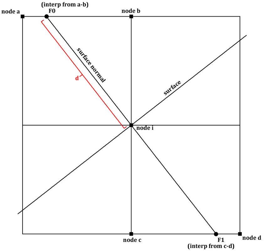
However, even with this information, I do not see an easy way to compute the derivatives across the interface in the normal direction using the gridded data. My best effort so far has been to project a line from each node, in the direction of the surface normal, until it intersects the edge of the local cell (see below). At this position the value of F is estimated by linear interpolation between nodes a and b. The same is done in the backward direction and using the known distance, the 2nd derivative at node i is found as
This part of the code is a big loop so I just explain it in this illustration:

I've compared my numerical prediction to the true value for the second derivative across the interface, which is:
My approach works okay, but it is not very precise, with errors that can be quite large (>5%).
Is there perhaps a better way to do this?? I planned to try cubic interpolation instead of linear interpolation to improve things, but maybe a different approach is better.
Code:
xnum = 100; % grid nodes in x direction
ynum = 100; % grid nodes in y direction

xgrid       =  (-(xnum/2-1/2):1:(xnum/2-1/2)) ;  x = repmat(xgrid,[ynum 1]); % grid distance in x direction
ygrid       =  (-(ynum/2-1/2):1:(ynum/2-1/2))';  y = repmat(ygrid,[1 xnum]); % grid distance in y direction
r =  sqrt(x.^2+y.^2); % distance from central node

L = 10; % thickness of diffuse interface
radii = 40; % radius of circle

F = 1-(1+sin((pi/L)*(r-radii)))/2; % create diffuse interface
F(r<(radii-L/2))       =  1; % create diffuse interface
F(r>(radii+L/2))       =  0; % create diffuse interface
What I want to do is, use numerical methods on the regular grid to get the best approximation of the second derivative of F in the direction normal to the interface, for every node within the interface. To start, I get surface normal components as
Code:
dfdy       =  abs(circshift(F,[1 0])-circshift(F,[-1 0]))/2; % first derivative of f in y direction
dfdx       =  abs(circshift(F,[0 1])-circshift(F,[0 -1]))/2; % first derivative of f in x direction
normy = dfdy./sqrt(dfdy.^2+dfdx.^2); % surface normal, y component
normx = dfdx./sqrt(dfdy.^2+dfdx.^2); % surface normal, x component
However, even with this information, I do not see an easy way to compute the derivatives across the interface in the normal direction using the gridded data. My best effort so far has been to project a line from each node, in the direction of the surface normal, until it intersects the edge of the local cell (see below). At this position the value of F is estimated by linear interpolation between nodes a and b. The same is done in the backward direction and using the known distance, the 2nd derivative at node i is found as
Code:
dfdn2 = (F0+F1-F*2)/d^2This part of the code is a big loop so I just explain it in this illustration:
I've compared my numerical prediction to the true value for the second derivative across the interface, which is:
Code:
dfd2actual = (1-2.*F).*((pi/L)^2/2)My approach works okay, but it is not very precise, with errors that can be quite large (>5%).
Is there perhaps a better way to do this?? I planned to try cubic interpolation instead of linear interpolation to improve things, but maybe a different approach is better.